Lec 6, Introduction to Probability-I

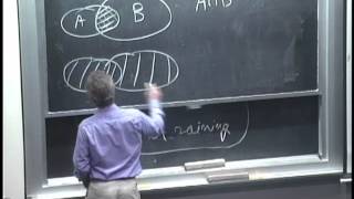
[Music] [Music] [Applause] [Music] [Applause] [Music] good morning students today we are going to next lecture lecture number six introduction to probability the concept of probability is fundamental any field whether you call it statistics or analytics are you data science everywhere because if you look at some of the book titles of the statistics and analytics it will come with probability and statistics because the concept of probability and statistics is you cannot separate it because always it go together because the concept of statistics since we are taking sampling we are predicting about the population so what will you be say with the help of sampling we have to attach always some probability because it cannot be 100% is sure that whatever you say with the help of sample will be exactly you cannot predict it so wins there is a prediction comes then you have to attach and probability to that okay today you'll see the it is introduction to probability I am going to I'm not going to teach in detail about that one what has ideas which are important for us only that I am going to teach so the lecture objective is to comprehend the different way of assigning probability understand and apply in marginal Union joint and conditional probabilities and solving problem using laws of probability including love addition multiplication and conditional probability and using a very important theorem that is the Bayes rule then to revise the probability at the end these are the my lecture objectives so we'll go the definition of the probability the probability is the numerical measure of likelihood that an event will occur the probability of any event must be been between 0 & 1 inclusively 0 to 1 for any even the sum of the probability of all mutually exclusive collectively exhaustive event is 1 later I will explain what didn't be mutually exclusive color to leox exhaust 2 events so always the the probability of summation of probability will be equal to 1 for example probability a plus probability B and probability C equal to 1 here a B and C are mutually exclusive and collective it's this is the range of probability you see that if is any impossible event the probability value zero if it is a certain event the probability is one but there's a 50% chance the probability is 0. 5 so the point here is it is the probability lies between 0 to 1 okay the method of assigning probability there are three methods one is the classical method of assigning probability rules and laws then relative frequency of occurrence that is the cumulative historical data and subjective probability there is a personal intuition or reasoning by using these three methods let us see how to find out the probability first what is a classical probability the number of outcomes leading to an event given by the total number of outcomes possible is a classical probability each outcome is equally likely that is equal chance of getting different outcome so it is determined a priori that is before performing the experiment we know what are the outcome is going to come suppose we toss a coin there are two possibility head or tail in advance we know what are the possible outcomes it's applicable to games of chance the objective is everyone correctly using the method assign an identical probability because what is happening here using classical probability that everyone will get the same answer for the problem because we know in advance what are the possible outcomes so mathematically the probability of e is enough Eder by capital n where the capital n is the total number of outcomes enough Yi is the number of outcomes in E then relative frequency probability it is based on the historical data because the another name for relative frequency is a probability it is computed after performing the experiment number of items and even occurred divided by number of trials nothing but frequency then divide sum of frequency here also everyone correctly using this method as saying as identical probability because everything is already known to you so the same formula probability is enough yield away enough we're a small any as number of outcomes capital illness total number of trials then subjective probability it comes from a persons into intuitions our reasoning subjective means different individuals may correctly assign different numerical probabilities to the same event it is the degree of belief sometimes subjective probability is useful for example if you introduce a new product suppose if you want to know the probability of success of the new product so we can ask an expert that what is the probability of success even it is a new movie or a new project what is the probability of success it is based on the intuition are based on the experience of the person he can give some probability of success or failure for example site select decisions for sporting events for example in cricket what is how much possibility of one team to win these are intuitive probability in this course that there are certain terminology with respect to probability you have to know it is very fundamentals even though you might have studied over previous classes it is just to recollect it what does the experiment we will see what is experiment event elementary when sample space the Union and intersections mutually exclusive events independent events collectively exhaustive events complementary events these are the some terms we will revise this one is we say what is experiment trial elementary event and event experiment a process that produces outcomes is experiment so there are more than one possible outcome is there only one outcome portrayal what is a trial one repetition of process is a trail what is the elementary event even that cannot be decomposed or broken down into other events that is elementary events then what is the event an outcome of an experiment may be an elementary event may be aggregate of elementary event usually represented by uppercase letters for example AE that is notation for event we look at this example if you look at the table there are some towns population is given there are four families their family ABCD we have asked two questions children's in household whether do you have children or not see family a yes then we asked number of automobiles how many number of automobiles you have three be they have children they have two automobile so the help of this table we will try to understand what is the experiment for example randomly select without replacement two families from the residents of the town for example randomly we can select so elementary event for example the sample includes family a and C randomly we are selected so even each family in the sample has children in the household the sample families only a total of four automobiles so these are particular events for example for event each family in the sample has children in the household for example a is one event D is another event for example the sample family is only a total number of for automobiles for example a and C they have four automobiles B and D they have four automobiles a and D they have more than four automobiles this is the example of event then what is the sample space the set of all elementary events for an agreement is called a sample space suppose if you roll your die there are you can get one two three four five six these as a sample space there are different methods for describing the sample space when is a listing tree diagram set builder notation and when diagram you will see what is that see this is listing experiment and Emilee select without replacement to families from the residents of the town so each ordered pair in the sample space is elementary even for example D comma C say what is different possibility look at this table a b a c ad b c b a b c BD c AC b c d so this are see listing the sample space what is that we have to select two families from the residents so here we are doing without replacement without replacement means suppose EA it won't be again a if it is a B it won't be again b1 so a is taken we are not selecting another EA so without replacement the same thing they another way to express the sample spaces with the help of diagram this is a tree diagram is very useful and easy to understand for example ABCD there are four families we can have competition a beam we can combination AC ad b a b c b d CA c b c d da DB DC so this is easy with these different sample space because tree diagram is easy to understand ok now the set notation set notation for a random sample of two families so s equal to open bracket X comma Y X is the family selected on the first draw and Y is the family selected on the second draw it is the concise description of large sample spaces in mathematics they use this kind of notations you see the sample space can be shown in terms of Venn diagram so this is a list of sample space see that this is a different dot express different sample space then we'll go to the another concept union of sets the union of two sets contains an instance of each element of the two sets for example X is 1 4 7 9 1 said Y is another set 2 3 4 5 6 so if we want to know X Union Y just we have to combine 1 2 3 4 5 6 7 8 9 similarly if you look at the Venn diagram X is 1 Y is 1 if you want to know a union combining both the events another example say see IBM Dec Apple that is the C set there is another study of apple grape lime suppose we want to know union of set C and F so we have to take IBM Dec Apple Apple is coming in both the sets we are taking only one grape like this is the union we will go for intersection suppose x equal to 1 4 7 9 1 set y is 2 3 4 5 6 if you want to know common intercepts is 2 sets contain only those element come so here the four is come for is common in x and y so X intersection y is for for example C and D F in see we have IBM DZ Apple in the FE of Apple grape lime the C intersection F that is a common thing between set C and F is Apple so this one say this this this portion says our intersection then we will go for mutually exclusive events even with no common outcomes is called mutually exclusive events occurrence of one event precludes the occurrence of other event for example C B mdz Apple F is a grape lime so C intersection there is no common thing so that is why it is a null set similarly X 1 7 9 Y is a 2 3 4 5 6 X intersection y there is no common said look at the the Venn diagram there is no common thing so X intersection y is 0 these two sets are not overlapping so it's called to meet you'll exclusive events another example for this when we toss a coin there's a two possibility to get the outcome one may be head or tail it cannot have both that's why both even sir mutually exclusive event then independent events so occurrence of an event does not affect the occurrence are non occurrence of other even is called independent event the conditional probability of x given Y is equal to the marginal probability of X the conditional probability of Y given X is equal to the marginal probability the one way we will do one small problem on this one way to test the independent event is suppose the p of x given y equal to P of X and if P of Y given X is P of Y then even x and y are called independent events we'll go in detail after some time but with the help of an example ok collectively exhaustive event it contains all elementary events for an experiment suppose E 1 e 2 u 3 sample space with the three collectively exhaustive events suppose for you roll your die all possible outcome 1 2 3 4 5 6 that is collectively exhaustive events then complementary events and elementary events not in the a or is its complimentary event you see that the P of Y a is there which is not there that is a - that is called a compliment is a P of a disease equal to 1 minus P of a then counting the possibilities because in probabilities many time different the combinations may come these rules may be very useful for counting different possibilities one rule is m and rule second one is sampling from me a population with replacement second one is sampling from your population without replacement will go for Yemen rule if an operation can be done M ways and the second operation can be done in ways then there are Yemen ways for the two operation to occur in order the rule is easily can be extended to K stages with a number of ways equal to if there are K stages n1 n2 n3 done for simply be able to multiply this for example tasks to kind the total number of sampling event is 2 multiplied by 2 equal to 4 because in the first kind you make a 2 possibility second kind you make it another 2 possibility so the total is 4 possibilities suppose you see that another example of sampling from a population with replacement one example is a tray contains a thousand individual tax returns if 3 returns are randomly selected with replacement from the tray how many possible samples are there so every time you are going for a 3 trial trial one trial to trial 3 in each trial there are thousand possibilities because you can choose one from thousand so first it trials thousand second times thousand third trial thousand when you multiply this this is thousand million possibility set with replacement in case if you go without replacement the same thing because the without replacement what will happen the sample size will decrease a tray contains thousand individual tax returns if three returns are randomly selected without replacement for the tree how many possible samples are there so that is a NC n that is the n factorial by n factorial little by n minus n factorial there's a thousand factor right three thousand minus 3 factorial it is one thousand six six two six million 160,000 you see the previously with replacement in a way to previous light with replacement it is a thousand million now it is only 166 million because we are going for without replacement there are different types of probability say we can call it as a marginal probability Union probability joint probability and conditional probability then what is the notation marginal probability is simple one probability P of X so how it is expressed in terms of Venn diagram see this this one so marginal probability then Union probability it is a X Union Y the probability of x ry counting's the joint probability our common probability the probability of x and y occurring together the middle portions then conditional probability the probability of X occurring given that Y has occurred here there are two event the probability of the outcome of X is depending upon the outcome of Y so we ought to read it probability of x given that Y has occurred so this is the Venn diagram notation for expressing the conditional probability then we will go for a general law of addition so P of X Union Y equal to P of X plus P of y minus P of X intersection Y will take on small example from that example will understand the concept of probabilities a company is going for improving the productivity of that particular unit they are coming with a new design one design is layout design for example layout design one design will reduce the noise that is one option there is a second design that will give you more storage space so we are going to ask from the employees what kind out of these two design which we'll improve the productivity okay you see the problem a company conducted a survey for the American Society of interior design in which workers were asked which changes in the office design would increase productivity there are two design is there one is the one design will reduce the noise another design will improve the storage space the responders were allowed to answer more than one type of design changes so this table shows the outcome so 70% of the people have responded that reducing nice would increase the productivity 67 percentage of the respondent have responded that more storage space would increase the productivity this is to design so we are asking the from the responder which design will improve the productivity suppose if one of the survey respondents were randomly selected and asked what office design change would increase workers productivity otherwise what is the probability that this person would select reducing noise are a design which is helpful for providing more storage space out of these that reduce out of two options so let n represents the event reducing noise that means using that design yes represents the event more storage space yes there is another options the probability of person responding to n are yes can be symbolized statistically as a union probability by using law of addition that is a P of en Union yes so see that P of n union s is because we know the as per the our the formula p of n unions is P of n plus P of s minus P of n intersection yes so the P of n is 70 percentage P of s is 67 percent age those who have told yes for both the designs is 0. 56 so when you substitute these values in the formula so we are getting 0.

81 there is 81 percentage of the people have told both the designs will increase the productivity what you are solved with the help of Venn diagram in previous in in in the previous slide can be solved with the help of contingency table this contingency table is so helpful just you had to make a table for example in in rows I have taken nice induction the noise reduction say 70% as people have told yes so remaining 30 metal told no 70 30 in the column I have taken increasing storage space design in the ATC 67 percentage total they have told that increasing storage space would increase the productivity so remaining 33 meter told no so the point 5 6 is intersection people have told both yes for both a design that is for nice reduction and increase in storage space so once if you know this point 5 6 the remaining things you can simply you can substrate it 0. 7 0 minus point 5 6 is point 1 4 that is those who are told no to storage space and yes to noise reduction then if you substrate from 0. 67 will get 0.

1 one 0. 33 - 0. 14 you will get 0.

19 so from this table we can read a lot of information whatever it has no this is for example even a a 1 a 2 even B 1 B 2 this in the rows you see that it is in the columns whatever cell inside the cell this portion is called join probabilities P of a1 intersection B 1 whatever it is the extreme side of the table see that this this is called marginal probabilities this is the notation that traditionally they follow whatever the inside the cell it is a combination of both the even that is the it is the joint probabilities whatever extreme it end it is a marginal probability extreme side of the table okay the same thing suppose if you if we want to know the same answer with the help of this contingency table we want to know how much percentage of the people who have a for both the design that is n and yes so P of n plus P of s minus P of N and s so this value directly we can read it from the table so P of n is 0. 7 plus P of s is 0. 67 minus P of Y n intersection is is 0.

56 so when you do that we get you point eight one then we will go for conditional probability the probability of n is 0. 7 0. 8 both the design end and yes is 0.

56 suppose if you want to know P off yes given n equal to P off again intersection yes doodled by P of n so this value I will explain this conditional probability in detail later but now you take this one so P of n intersection yes from the previous table you can find out the point five six even look at the Venn diagram also P of n is 0. 7 when you substitute we're getting 0. 8 the same office design problem you see that there is another conditional probability P of n - given Y that means those who are told no to noise reduction but they are agreed for storage design so this is the conditional probability so we ought to multiply P of n - intersection yes it'll be P of s n - intersection a says this point because en no yes this is a point 1 1 Deuter by PF is 0.

67 that is equal to 0. 16 for Realty we'll take another small problem will explain the concept of probabilities with the help of the problem a company data revealed that 155 employees work it on 4 type of positions the table is shown in the next slide raw value of matrix also called contingency table with the frequency counts of each category and subtotals and totals containing breakdown of these employees by type of position and by sex you see that look at this table in rows the type of position they hold in their organization whether they are working in a managerial position professional or technical or clerical in the column sex whether male or female you see the intersection of managerial and male eight that represents both that is the wor managerial or working in a managerial position the same time they are male so that is our joint values in here the only count join counts the extreme right are the bottom of the table we have given the total counts now if any employee of the company is selected randomly what is the probability that the employees female or professional worker so what we have to do so we are going to find out P of F in Union peel that is a P of F plus P of P minus P of F intersection P so P of e FA is when you go to the previous one P of F is so when you divide 55 by 155 you will get 0. 3 35 P of P is when you divide 44 daughter by 155 you will get to 0.

8 to 4 minus P of F intersection P that is F intersection P 30 13 tutor by 155 you will get point 0 8 4 that equal to 0.