Lec 9, Probability Distribution - II

Data Analytics with Python Prof. Ramesh Anbanadham Department of Management Studies Indian Institute of Technology – Roorkee Lecture - 09 Probability Distribution – II Dear students in this lecture, we are going to see some of the discrete distributions and continuous distributions, the discrete we are going to study the binomial poisson hypergeometric in continuous that where we going to study uniform exponential and normal, first you will see, what is the application of this Binomial Distribution? Otherwise what is the need of this binomial distribution.

We will take one practical example that I will solve manually with the help of our concept of probability then I will tell you how the concept of binomial distribution will help us to solve this problem quick way, but just consider the purchase decision of the next 3 customers who enter your store and the basis of past experience. The store manager estimates the probability that any one customer will make your purchase is 0. 30.

Now, what is the probability that 2 of the next 3 customers will make a purchase? That problem is drawn in the form of a tree diagram the first customer, second customer, third customer when the first customer comes, there are 2 possibility he can go for purchase or not purchase, purchase mention as say S success failure. The second customer also may go for purchase, not purchase third customer purchase, not purchase.

Look at the first possibility the First customer is purchasing, so, success, success, success that is S, S, S. If you take X look at the bottom of this slide, if X equals the number of customers making a purchase, so, in this category, all 3 customers all 3 are going to buy look at the second possibility success, success failure. So, in this out of 3 customers 2 customers S S going to purchase like this we have displayed all possibilities.

Now, the problem is X what is asked is 2 out of 3 customers what they have purchased. So, number of customers making a purchases how many possibilities are there 2 customers 1, 2, 3 how we got this 3 is nothing but your 3 C 2 the 3 C 2 is out of 3, what is the probability? What is the chance that 2 customers will buy there will be a possibility of 3 C 2, so the 3 C 2 is 3.

Now, we will see the first customer all possibilities purchase purchase no purchase success success, so, success we know, we are calling it is a p failure is 1 - p. So, it is a p 2 into 1 - p p is (0. 30)2 multiply by 0.

70, it is a 0. 63. For second chance also first customer may buy second customer did not buy third customer also buy, so, it is success failure success.

So, p 1 - p into p again p2 into 1 – p, 0. 063, third choice, no purchase purchase purchase FSS, so 1 - p, p,p so it is a p2 . (1 – p) = 0.

63. If I plot this one see x possibility, x possibility this possibility is see this possibility, when x = 0, that means, what is the charge that all 3 customers will not buy? That is this case 0.

7, 0. 7, 0. 7.

If I say x = 1, what is the probability that 1 customer will buy, if x = 2? What is the probability 2 customers will come, 2 customers will buy with x = 3? What is the probability that 3 customers will buy?

So, we can do with the concept of probability manually like this. So, the question is asked is this one? What is the probability that 2 customers will buy out of 3.

So, this is your probability distributions. So, this we can do manually but it will take a lot of time. So, here with the help of your binomial distributions, you can get right this all possibilities going back this way nC x So, p ( X=2) = nC x p power x q power n - x, where n = 3 where x = 2 p is the probability success q = probability of failure.

So, this nC x will give you different combinations of that event to happen. So, this p power x see that always here p2 q n - 2. So, this will give you the probability.

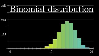
So, that is the purpose of this binomial distributions. What is the property of this binomial distribution experiment involves in identical trials, each trial has exactly 2 possible outcomes success, failures. Each trial is independent of the previous trial for example, the previous case customer one may buy or may not buy.

That is not depending upon the for example for the second customer is intension of purchase is not based on the previous customer. So, p is the probability of success on any one trial, the q is probability of failure on any one trial. So, p and q are constant throughout the experiment, this is important assumption.

So, x is the number of success in the end trials, there the previous case we are seeing x = 2. So the probability function as I told you can written as nC x that is nothing but n factorial divided by x factorial into n - X factorial p power x q power n - x the mean of this distribution is mu = n into p directly we are going to answered. So, you can find out I think but using the concept of expected value, when you multiply this p of x with the x, sigma of x into P of x, when you simplify will get this formula.

Similarly, variance directly we are going to use only the result variance equal to nPq standard deviation is root of nPq. Sometime there is ready made table is there to find out binomial probability values for example, n = 10 and n is number of trials, x = 3 , p = 0. 04 , n = 10 , x = 3 that value is this one 0.

150. So, the tables are provided you do not use your calculator it may take more time. Now we will find out mean and variance suppose, for the next month the clothing store forecast 1000 customers will enter the store the previous problem their 1000 customers.

So, what is the expected number of customers who will make the purchase out of 1000. So, the answer is mu = n into p so n this 1000 probability of success point 3, so it is equal to 300. So, that is out of 1000 customers, there is a chance that 300 customers will make the purchase.

For the next 1000 customers entering the store the variance and standard deviation of the number of customers who will make the purchase can you written as npq. So, n is given p is given 1 - p 70 210 the standard deviation is 14. 49.

Then will go to next distribution Poisson distribution describes discrete occurrences over continuous or interval. Generally Poisson distribution is for rare events, it is an discrete distribution. X can have only few discrete values.

Yes, it describes the rare events, each occurrence is independent of any other occurrences. The number of occurrences in each interval can vary from 0 to infinity. The expected number of occurrences must hold constant throughout the experiment.

These are the assumption of Poisson distribution. Some of the examples are application of Poisson distribution. So, arrival at the queuing system follow Poisson distribution, any airport people may arrive, airplane may arrive automobile may arrive, baggage may arrive that follow Poisson distribution.

The banks people automobiles loan applications this arrival pattern follow Poisson distribution in computer file services, read and write operations will follow Poisson distribution The defects in manufacturing goods can be considered an example of Poisson distribution. For example, number of defects per 1000 feet of extruded copper wire see that the n is very large. The probability of success is very low.

Another example of Poisson distribution is number of blemishes per square foot of painted surface blemishes kind of a defect in paint number of errors per typed page, these are the example of your Poisson distributions. So, the probability function for Poisson distribution is lambda power X e power - lambda divided by X factorial, where X can take only discrete value, the lambda is mean that is a long run average the value of e is 2. 71.

The mean of this Poisson distribution is lambda variance of the Poisson distribution lambda standard deviation of Poisson distribution is root of lambda. So, this distribution called the univariate distribution. Because it has unique parameter that means, it is a special property of your Poisson distribution where mean and variance is same.

So, that is mean and variances. Same that is lambda. And another caution while using Poisson distribution is the unit of this lambda and X should be same, for example, lambda equal to 3.

2 customers for 4 minutes probability of around 10 customers in 8 minutes. So, you have to adjust the lambda, how will you adjust, you multiply by 2, so it will be 6. 4 into 8.

Now, the unit of X and lambda is same, then you can use your probability function, P of X = lambda power X and e power – lambda and substitute X = 10. We are getting 0. 025.

See the second one, lambda = 3. 2 customers by 4 minutes, X = 6 customers for 8 minutes. So, you have to multiply lambda.

So, it will be 6. 4 in 8 then P of X will get the answer. So, what is the point here is the unit of lambda and X should be same.

Here also there is a probability Poisson probability table is available. So, when Mu = 10 X = 5, you see in the column shows mu. So, Mu = 10 here, X = 5 is this value.

So, this value is 0. 378. So, you cannot, you need not to use your calculator directly you can read it from the table.

But we are going to use these things in your practical class we are going to find out probabilities with the help of Python. We will go for hypergeometric distribution, see the binomial distribution is applicable, when selecting from finite population with replacement or for an infinite population without replacement. So, whenever the concept of without replacement comes, then we have to think of using hypergeometric distribution.

The hypergeometric distribution is applicable when selecting from your finite population without replacement. The properties of hypergeometric distribution, so, sampling without replacement from your finite population then you should go for hypergeometric distribution. The number of objects in the population is denoted as N, each trial has exactly 2 possible outcomes, success or failure.

Similar to binomial distribution trials are not independent, this is one different property, when compared to binomial. In the binomial distributions, since we are going with replacement, the trials are independent; here we are going without replacement. So, the trials are not independent, it is dependent.

Then, that means, the P will not be fixed, the probability of P will not be fixed, every time we will get different answer for the P. X is the number of success in the n trials. The binomial is acceptable approximation N divided by 10 is greater than or equal to n, otherwise, it is not.

That we will see the probability function with discrete values use probability mass function, if it is a continuous will use PDF probability density function. So, the probability mass function is P(x) = (ACx) (N - AC n – x) / NCn. So, here see the capital letters represent for the population.

So N is for population size, A is the number of success in the population, small letter, n for the sample size, the x is number of success in the sample. So, P(x) = (ACx ) (N – A C n – x )/ NCn. The mean value is A into n / N.

The variance and standard deviation of hypergeometric distribution is A N - A n into N – n / N square into n – 1, root of sigma squared is the formula for standard deviation. Will see one problem here, different computers are checked from 10 in the department, 4 out of 10 computers have illegal software loaded. What is the probability that 2 of the 3 selected computers will have illegal software loaded.

By looking at the problem we are feeling that it is a finite population. Whenever there is a finite population, we should think of hypergeometric distribution. So, N is given that N is your population size, A is 4, because we know 4 is out of 10, 4 computers are illegal software.

Because we know the how much illegal software is installed in the population A = 4. Then, what is the probability that x is 2 of the 3 selected the computers will have illegal software loaded. So, x = 2, here n is 3 there are 2 things is there, one is for the population and population N = 10, A = 4.

For the sample n = 3, then what is the probability of that 2 out of 3 selected computers will have illegal software loaded. So now substituted, everything is given, so we will get 0. 3.

So what is the meaning of this 0. 3, the probability that 2 of the 3 selected computers will have illegal software loaded is 30%. Then we will go to the continuous probability distributions.

A continuous random variable is a variable that can assume any value in the continuum. That is, can assume an uncountable number of values. Thickness of an item, time required to complete a task, temperature of a solution, height, these are example of continuous random variable.

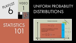
This can potentially take any value depending only on the ability to measure precisely and accurately. First we will see uniform distribution. The uniform distribution is the probability distribution that has equal probabilities for all possible outcomes of a random variable.

That is the probability of random numbers also. When we say random numbers, the probability of choosing any number is same, because of its shape, it is also called a rectangular distribution. Look at this, Uniform Distribution.

The uniform distribution is defendant interval, a less than equal to x less than equal to b. So the probability function is 1 divided by b - a, where ‘b’ is upper limit, ‘a’ is the lower limit. In other interval, the value of f (x) is 0, the area = 1.

The mean of a uniform distribution is Mu= a + b divided by 2, standard deviation is b - a divided by root of 12. These very standard result, the derivation of this one, you can refer some textbook. Now, we will see some problem using uniform distribution, suppose uniform probability distribution over the range is defined this way.

2 less than or equal to x less an or equal to 6. So if you want to know f of x we know that 1 divided by b - a b is 6, a is 2, so, 1 divided by 6 - 2 is 0. 25.

What is the meaning of this 0. 25 means, in between 2 and 6, you can select any random variable, maybe 3, you may select 3 or 4 or 5, the probability of choosing 3 or 4 5 is, 0. 25.

So, the mean is a + b by 2 is 4 a is 2 b is 6 8 divided by 2 is 4. Similarly, standard deviation is b - a whole square divided by 12 that is 1. 17.

We will see another example, suppose a random variable is defined between 41 to 47. First, we have to find out probability density function 1 divided by b - a, so 47 - 41, so that is 1 / 6. So 1 / 6 the height of this rectangle of distribution is 1 / x this value is your 1 / 6.

The lower limit 41 upper limit 47. So, the mean of the distribution is 41 + 47 divided by 2 so 88 divided by 2 44 standard deviation is b - a root of 12. So, 47 - 41 root of 12 is 3.

464 it is 1. 732. Now, see the uniform distribution is defined in this interval 41 to 47 right.

Suppose, we want to know the probability between 42 and 45, is it 42 and 45. So, that had not been done by 45 x that is x2 - x1 divided by b - a ,x2 is 45 x1 is 42 So, 45 - 42 is 3 divided 6 divided by 6 is 1 / 2. So, this area is 0.

5. You will see another example of this uniform distribution. Consider a random variable x representing the flight time of an airplane travelling from Delhi to Mumbai.

Suppose the flight time can any value in the interval between 122 to 140 minutes. Because of the random variable x can assume any value in the interval, x is a continuous rather than a discrete random variable. Let us assume that sufficient actual flight data are available to conclude that the probability of your flight time within any one minute interval is the same as the probability of a flight at time within any other one minute interval, contained in the large interval from 120 to 140.

So, that is the properties of your uniform distribution. That means, in any one, any small interval you should have the same value. If any one interval, if any between this interval the probability will say next, another one minute interval, the probability same.

With every one minute interval being equally likely the random variable x is set to have a uniform probability distribution. So, the upper limit is 140, the lower limit is 120 1 divided by 140 - 120 is 20. So, the height of this rectangle distribution is 1 divided by 20, it is starting a value is 120, b value is 140.

Suppose, you are asked to find out, probability of your flight time between 120 and 130 minutes. So, somebody is asking what is the probability of that, flight arriving between 120 and 130 minutes. So, what you have to do, this is 130 - 120 divided by 140 - 120.

When you simplify you will get 0. 50. So the probability of that flight arrive between 120, 130 minutes is 50%.

Next we will go to the exponential probability distribution. The exponential probability distribution is useful in describing the time it takes to complete a task. The exponential random variable can be used to describe the time between vehicle arrivals at a toll booth, time required to complete a questionnaire, the distance between major defects in a highway.

For example, whenever the time between arrival and time required to complete the questionnaire, whenever the word the between comes. Then that is the then it is appropriate to use exponential distribution. The density function for a exponential probability distribution is f of x = (1 divided by Mu).

e to the power - x divided by Mu. Mu is the mean. We will see what is the how to construct the exponential distribution.

Suppose that x represents the loading time for a truck at a loading dock and follow such a distribution. If the mean or average loading time is 15 minutes, Mu = 15, then appropriate probability density function is f of x = 1 divided by 15 e to the power – x divided by 15. So, what is the meaning of this exponential distribution is supposed, if the loading time, the probability of loading time less than 6 is this area.

The probability of loading time between 6 and 18 is this one this time, this is a probability, this shadowed portion represents the probability of that loading time is between 6 and 18. Because in many application of exponential distribution will use the cumulative probability density function. So, for an exponential distribution, the formula for finding the cumulative probability density function is 1 - e to the power - x 0 / Mu where x0 is some specific value of x.

it is nothing but if you integrate that to distribution, if you integrate the distribution between the intervals when you simplify it, you will get this answer. We will see one example of this exponential probability distribution. The time between arrivals of cars at a petrol pump follows an exponential probability distribution with the mean time between arrivals of 3 minutes.

See that it is mean time between arrivals. So, the mean is 3 here. The petrol pump owner would like to know, the probability that time between 2 successive arrivals will be 2 minutes or less.

So x value is less than or equal to 2. So if you want to know P of x less than equal 2, we have to substitute into the, that distribution. That is the cumulative to distribution function, 1 - x value, so it is 0.

4866. It is a 0. 4866 so this one.

So this shaded one. Suppose if you want to find out, the time between 2 successive arrivals of vehicle is less than 7 minutes, probability will increase. So, when x increases, but there are more chances that the time between 2 success arrival is this much.

So what I am saying this is a way to interpret the exponential distribution. Now, there is a very important relationship between poisson and exponential distribution. See, the Poisson distribution provides an appropriate description of number of occurrences per interval.

So, one interval is there. In that interval, how many occurrences happened, that is the Poisson distribution. In the exponential distribution provides an appropriate description of length of the interval between the occurrences.

Suppose the same interval between this occurrence to this occurrences, so this phenomena is explained with the help of between 2 occurrences, this phenomena is explained with the help of exponential distribution. Number of occurrences in that interval it is explained with the help of Poisson distribution, that is a relation between poisson and exponential distribution. So, mean of your poisson and mean of your exponential distribution, what is the relationship.

Because the average number of arrival is 10 cars per hour, the average. So, if it is a 10 in that interval, there are 10 cars are arriving. So, this mean is taken for the Poisson distribution.

But 1 / 10 is taken as the mean for the exponential distribution. That means, time between arrivals. So, that is a link between Mu generally we write Mu mean for Poisson distribution, 1 / Mu mean for exponential distribution that is the relation between poisson and exponential distribution.

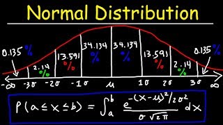
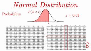
Next, we are entering into the very important distribution that is a normal distribution, normal distribution is we can say a father of all the distributions. Because suppose some phenomena is happening if you are not aware, you can assume that it follows normal distribution. Normal distribution is following Bell Shaped, it is symmetrical, mean, median and modes are equal.

The location of the normal distribution is characterized by Mu, the spread is characterised by Sigma. The random variable has an infinite theoretical range that is minus infinity to plus infinity. The density function of a normal distribution is f of X = 1 divided by root of ( 2 .

pi . sigma) . e to the power - 1 / 2 x - mu by sigma whole squared, e is mathematical constant value is 2.

71, pi is the mathematic constant we know that 3. 14, Mu is the population mean, Sigma is the population standard deviation, X is any value of the continuous variable. The shape of the normal distribution is by varying the parameter of Mu and Sigma we obtained different normal distributions.

Dear students, what we have seen so far is we have seen some of the discrete and continuous distributions in the discrete distribution we have talked about the binomial, poisson distribution. In the continuous distribution we have seen exponential and uniform distributions. The next class very important distribution that is normal distribution, that will cover in the next class.

Thank you very much.