Designing a Lag Compensator with Root Locus

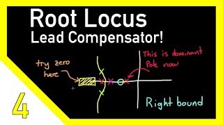
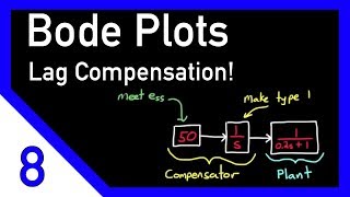
welcome back to control system lectures this video will focus on designing phase lag compensators using the root Locus method if you're watching my videos in the order of one of the playlists I've created then you've probably just watched the video on designing a lead compensator using the root Locus method which is good because I'm going to continue from where I left off there if you came to this video by another means then you might want to first check out that other video now I've already let on that the only difference between a phase lead and phase lag compensator is whether the zero or the pole is closer to the origin the zero for phase lead or the pole for phase lag or another way of saying it is whether the time constant to is larger in the numerator or the denominator so you might be thinking well if the transfer function is practically the same basically just a constant has been changed then can't I use the exact same techniques for Designing both lead and lag compensators and yes you absolutely can I showed in the last video that the purpose of phase lead is to move the poles further into the left half plane here is a simple root locus of an uncompensated two-pole system when we add a lead compensator to the system we are effectively dragging those two yellow lines more to the left where the pink lines are we usually are doing this to make the system more stable have a faster rise time and so on but in the root Locus method the bottom line is that we're trying to move the D dominant poles to the location in the S plane where our requirements want them for example we want to move the red poles to the green pole location with a lead compensator you might refer to this as shaping the root Locus plot or actually moving the lines around on the plot so if for some reason you want your dominant poles closer to the imaginary axis then you can use a phase lag compensator to reshape the root Locus like this in the exact same manner typically though this isn't what you use a lag compensator for sure there can be some advantages to moving the roots to the right but I'll discuss them in the lag compensator with bod plot video coming up next in general we use the lag compensator to address steady state errors for example maybe you want to look at the error of a unit step input response at time equals to Infinity but the trick is to address these steady state errors without changing the locations of the dominant poles since they're already where you want them as a consequence you don't want to shape the root Locus at least not by very much so you want to add the lag compensator in such a way that won't affect the shape of the root Locus and I'll explain how to do that but first let me cover how the live compensator reduces the steady state error if you've watched various videos on this topic or read various books you'll notice that there are a lot of simple equations that can help you remember how to design a lag compensator the problem for me though is that there are multiple different ways of approaching this problem and I tend to get my helpful equations all mixed up and in the end I end up messing up the problem like for example does the a multiply across the entire numerator or just the first s and since I always forget these little helpful equations I end up just starting from scratch and do it the long way that way you're sure not to use the wrong equation and you'll probably have a better understanding in the process let me draw a generic transfer function for a plant G of s but to make it easier in the future I'm going to break this up into a numerator GN and a denominator GD I'll also add a lag compensator s- Z over s minus P remember the locations of the zeros and poles are negative since they're in the left half plane so these will become Z plus a real number I'll feedback the output and compare it against a reference U of S to generate an error term e of s now from my video on steady state error you know that the equation for or ESS or steady state error of a plant G of s is the limit as s approaches zero of U of S over 1 + G of s and for a step input U of S is just 1 / s so this equation just becomes the denominator of G when s equals 0 divided by the denominator plus the numerator of G when s equals 0 so now when we add the lag compensator in the system we can solve for the new steady state error I'll call it ESS of C for the steady state error of the compensated system now the total system is G of s times the lag compensator and again for a step input U of S equal 1 /s and the whole equation just becomes this notice that it is very similar to the uncompensated equation but just with that extra pole and extra zero multiplied in we can solve for the ratio of the zero to the pole and get this equation now essc is the desired steady state error to a unit step input and we can pick almost any value we want for this we know the uncompensated plant G of s and so now we can determine the ratio of the zero to the pole for our lag compensator that will get us the steady state error that we want from this equation though it's easy to see that in order to reduce the steady state error to zero or basically have no steady state error the zero to pole ratio would have to be infinite that's why a lag compensator can only reduce the error and not eliminate it if you want to eliminate it completely you'll have to increase the system type which means add a single pole at the origin let me show you a quick example with some arbitrary numbers let's say you have this plant and you want to add a lag compensator to reduce the steady state error to 0. 1 then the zero to pole ratio needs to be 13. 5 to 1 or in other words the zero needs to be 13.

5 times further away from the imaginary axis as the pole but where do we place them I mean we can place the pole at Min -. 1 and the zero at minus 1. 35 and satisfy that ratio but we could just as easily place the pole at minus one and the zero at -3.

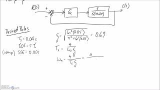
5 there is an infinite number of possibilities still to help us decide we first need to remember that a point in the S plane exists on the root Locus if the sum of the angles from the real axis to the line that extends from the pole or zero to that point equals 180° you add the angle if it's a pole you're measuring from and you subtract it if it's a zero so in this case we know that this blue dot exists on the root Locus if these two angles Theta 1 and Theta 2 add to 180° so if I don't want to move the location of the locus very much when we add a lag compensator then the angle of the added pole minus the angle of the added zero need to be very very close to zero so we want to place the pole and zero in such a way that they cancel each other out and there is no root Locus shaping if we place the lag compensator somewhere to the left of the dominant poles then you can see graphically that the angle of the zero is going to be much smaller than the angle of the pole this is going to drag the dominant poles to the right like I explained earlier on however if we move the lag compensator closer and closer to the imaginary line but still keep the exact same ratio then the angles for the pole and zero become closer and closer together and our condition is met so the bottom line when you're using a lag compensator to reduce steady state error is this maintain the zero to pole ratio that you've calculated that will reduce your steady state error to the amount that you want and then place the pole in zero as close to the imaginary axis as possible to reduce moving the dominant po but there is a limit to how far to the right you can move the compensator and that's because if you're building this with resistors and capacitors the closer to the imaginary axis you make this the larger the components need to be and eventually they becom so large as to be impractical so the rule of thumb is to place the zero approximately 50 times closer to the imaginary axis as the closed loop dominant pole of course this is just a rule of thumb so this is a place where you have a little bit of flexibility in the design so for example if you had your dominant poles at1 at the real axis like we have here then you'd want to place the zero at . 02 and then the pole at whatever the ratio is that is needed to meet your steady state error in the last video we designed a lead compensator for a system in order to move the dominant po from min-1 and-3 to a complex set of poles at-3 and plus orus 2 on the imaginary line now I've redrawn the complete closed loop system and compensator here and if we solve for the steady state error to a unit step input for this system we get approximately. 3 that means that if we input a step of one then at time equals infinity the output would only be 7 but let's say you have a requirement to have the steady date error be reduced to 0.

1 but you need to keep the dominant poles where they are in order to meet your performance requirements to an Impulse input so you go through the process of Designing a lag compensator and you find that the zero to pole ratio needs to be around 3. 8 and you know that the real portion of the closed loop dominant pole is minus 3 since you designed it that way so you find that you need to place the zero at . 06 and the pole 3.

8 times closer than that at16 so your lag compensator simply becomes s + 06 / s +16 and you can place it in line with your lead compensator and your requirements will be met now I went ahead and plotted the step response and the impulse response for this system in Matlab and placed the plots here you can see from the step response that the lead only system produced a steady state error of around. 3 just like we calculated and when we added the lag to it it reduced that steady state error to about 0.