Logistic Regression Details Pt1: Coefficients
944.28k views2606 WordsCopy TextShare
StatQuest with Josh Starmer
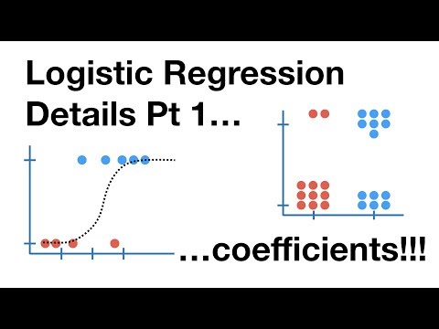
When you do logistic regression you have to make sense of the coefficients. These are based on the l...
Video Transcript:
If I were in Hawaii I'd be sitting on a beach In the shade of a tree Watching snack quest Hello, I'm Josh Starmer and welcome to StatQuest today We're gonna cover logistic regression and we're gonna dive deep into the details. This is part one of a series of videos I'm gonna do on logistic regression this time we're talking about coefficients This stat quest follows up on logistic regression clearly explained Which provides the big picture of what logistic regression is and how it works In this video. I want to dive deeper into how logistic regression works Specifically we'll talk about the coefficients that are the results of any logistic regression We'll talk about how they are determined and interpreted we'll talk about the coefficients in the context of using a continuous variable like weight to predict obesity and We'll talk about the coefficients in the context of testing if a discrete variable Like whether or not a mutated gene is related to obesity Before we dive into the details Let's do a quick review of some of logistic regressions main ideas to make sure we're all on the same page in This example the y-axis is the probability a mouse is obese It goes from 0 the mouse is not obese to 1 the mouse is obese The dotted line is fit to the data to predict the probability a mouse is obese given its weight If we wait a heavyweight Mouse Then the corresponding point on the line indicates that there is a high probability close to one that it is obese and if we weight a middleweight Mouse Then there's an intermediate probability close to 0.
5 that it is obese Lastly a lightweight Mouse has a low probability close to 0 of being obese Ok, those are all the basics we need for this stat quest One last thing before we get started I want to mention that logistic regression is a specific type of generalized a linear model often abbreviated GLM Generalized linear models are a generalization of the concepts and abilities of regular linear models Which we've already talked about in many stat quests That means that if you're familiar with linear models, then you are well on your way to understanding logistic regression We'll start by talking about logistic regression when we use a continuous variable like weight to predict obesity This type of logistic regression is closely related to linear regression a type of linear model So let's do a super quick review of linear regression Shameless self-promotion if you're not already familiar with linear regression Check out the stat quests on linear regression and linear models part one Ok, we start with some data and we fit a line to it and this is the equation for the line It has a y-axis intercept and a slope and We plug in values for wait to get predicted values for size So even though we didn't measure a mouse that weighed 1. 5 we can plug 1. 5 into the equation and predict that Mouse to have size 1.
9 1 And a mouse with weight 1. 5 and size 1. 9 one would end up on the line at this point Now even though it's silly the equation can predict the size of mice with weight equals zero that's just the y axis intercept zero point eight six and We can even predict the size of mice with negative weights I'm pointing this out because the fact that we are not limiting the equation to a specific domain and range makes it easier to solve and This has a big effect on how logistic regression is done So over on the left side we have the linear regression and on the right side we have the logistic regression with linear regression the values on the y-axis Can in theory be any number?
Unfortunately with logistic regression the y axis is confined to probability values between 0 and 1 To solve this problem the y axis in logistic regression is Transformed from the probability of obesity to the log odds of obesity. So just like the y axis and linear regression It can go from negative infinity to positive infinity So we can see what we're doing let's move the logistic regression to the left side Now let's transform the y-axis from a probability of obesity scale to a log odds of obesity scale We do that with the logit function that we talked about in the odds slash log odds stat quest P in this case is the probability of a mouse being obese and Corresponds to a value on the old y axis between 0 and 1 The midpoint on the old y axis corresponds to P equals 0. 5 and When we plug P equals 0.
5 into the logit formula and do the math We get 0 the center of the new y axis here Is P equals zero point 7 31 on the old y axis if? We plug P equals zero point seven three one into the logit function and do the math we get one on the new y axis if We plug P equals zero point eight eight into the logit function and do the math we get two on the new y axis if We plug P equals zero point nine five into the logit function and do the math We get three on the new y axis Lastly these blue points from the original data are at P equals one If we plug P equals one into the logit function and do the math Well, technically you can't divide by zero. However the log of one divided by zero equals the log of one minus the log of zero and the log of zero is defined as negative infinity and Since something minus negative infinity equals positive infinity this whole thing is equal to positive infinity This means the original samples that were labeled obese are at positive infinity on the new y-axis as a result the original y-axis from 0.
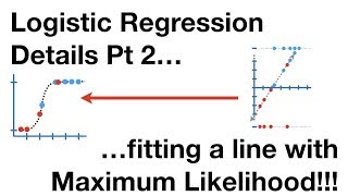
5 to 1 is Stretched out from 0 to positive infinity on the new y-axis Similarly 0. 5 to 0 on the old y-axis is stretched out from 0 to negative infinity on the new y-axis Ultimately we end up with the log of the odds of obesity on the new y-axis And the new y-axis transforms the squiggly line into a straight line The important thing to know is that even though the graph with the squiggly line is what we associate with logistic regression The coefficients are presented in terms of the log odds graph In the stack quest logistic regression details part 2 fitting a line with maximum likelihood We'll talk more about how this line is fit to the data But for now just take my word for it that this is the best fitting line Just like with linear regression the best fitting line has a y-axis intercept and a slope The coefficients for the line are what you get when you do logistic regression The first coefficient is the y-axis intercept when weight equals zero It means that when weight equals zero the log of the odds of obesity are negative three point four seven six in Other words if you don't weigh anything the odds are against you being obese, duh here's the standard error for the estimated intercept and The Z value is the estimated intercept divided by the standard error In other words, it's the number of standard deviations. The estimated intercept is away from zero on the standard normal curve That means that this is the Wald's test that we talked about in the odds ratio stat quest Since the estimate is less than two standard deviations away from zero.
We know it is not statistically significant and This is confirmed by the large p-value the area under the standard normal curve That is further than one point four seven standard deviations away from zero The second coefficient is the slope It means that for every one unit of weight gained the log of the odds of obesity increases by one point eight to five Here's the standard error for the slope Again, the Z value is the number of standard deviations. The estimate is from zero on the standard normal curve and Again, the estimate is less than two standard deviations from zero. So it is not statistically significant, this is no surprise with such a small sample size and This is confirmed with the large p-value Double bam Now we know all about the logistic regression coefficients when we use a continuous variable like weight to predict obesity now let's talk about logistic regression coefficients in the context of testing if a discrete variable like whether or not a mouse has a mutated gene is related to obesity on the left side we have mice that have a normal gene and On the right side.
We have mice with a mutated gene Just like before some of the mice are obese in some of the mice are not obese This type of logistic regression is very similar to how a t-test is done using linear models So let's do a quick review of how a t-test is done using linear models Shameless self-promotion If you're not already familiar with how a t-test can be performed using a linear model then check out the stat quest linear models part two t-tests and anova Okay, we start with some data in this case we've measured the size of mice that have a normal gene and the size of mice with a mutated version of that gene Then we fit two lines to the data the first line represents the mean size for the mice with the normal copy of the gene the Second line represents the mean size of the mice with the mutated copy of the gene These two lines come together to form the coefficients in this equation the mean value for size for the mice with the normal copy of the gene goes here and The difference between the mean size of the mice with a mutated gene and the mean size of the mice with the normal gene goes here We then pair this equation with a design majors to predict the size of a mouse Given that it has the normal or mutated version of the gene This is the design matrix for the observed data The first column corresponds to values for b1 and it turns on the first coefficient the mean of the normal mice The second column corresponds to values for b2 and turns the second coefficient the mean of the mutant mice minus the mean of the normal mice off or on Depending on whether it is a zero or a one For example the first row in the design matrix corresponds to a mouse with a normal copy of the gene We predict its size by replacing b1 with 1 in replacing b2 with 0 and then we just do the math and We see that this mouse is associated with the mean of the normal mice This row in the design matrix corresponds to a mouse with the mutated gene We plug in 1 for b1 and Plug in 1 for b2 and we see that the mean of the mice with the normal gene plus the difference between the two means Associates this mouse with the mean for the mice with a mutated gene When we do a t-test this way we are basically testing to see if this coefficient The mean of the mutant mice minus the mean of the normal mice is equal to zero But you already know all this t-test stuff what you really want to know is how it applies to logistic regression The first thing we do is transform the y-axis from the probability of being obese To the log of the odds of obesity Now we fit two lines to the data For the first line we take the normal gene data and Use it to calculate the log of the odds of obesity for mice with the normal gene Thus the first line represents the log of the odds of obesity for the mice with the normal gene Let's call this the log of the odds for gene normal We then calculate the log of the odds of obesity for the mice with the mutated gene Thus the second line represents the log of the odds of obesity for a mouse with the mutant gene Let's call this the log of the odds gene mutated These two lines come together to form the coefficients in this equation the log of the odds gene normal goes here in the difference between the log of the odds gene mutated in the log of the odds gene normal goes here and since subtracting one log from another Can be converted into division this term is a log of the odds ratio It tells us on a log scale how much having the mutated gene Increases or decreases the odds of a mouse being obese Okay, now that we know what the equation is all about let's substitute in the numbers the log of the odds for gene normal is just the log of 2 divided by 9 and The log of the odds for gene mutated is just the log of 7/3 Now we just do the math and that gives us these coefficients and Those are what you get when you do logistic regression the intercept is the log of the odds for gene normal and The gene mutant term is the log of the odds ratio That tells you on a log scale how much having the mutated gene increases or decreases the odds of being obese and here are the standard errors for those estimated coefficients and Here are the z values aka the Wald's test values that tell you how many standard deviations The estimated coefficients are away from 0 on a standard normal curve The Z value for the intercept negative 1. 9 tells us that the estimated value for the intercept negative 1. 5 is less than 2 standard deviations from 0 and thus not significantly different from 0 and this is confirmed by a p-value greater than 0.
05 The z-value for gene mutant the log odds ratio that describes how having the mutated gene Increases the odds of being obese is greater than two Suggesting it is statistically significant. And this is confirmed by a p-value less than 0.
Related Videos

15:12
StatQuest: Linear Discriminant Analysis (L...
StatQuest with Josh Starmer
792,962 views
10:23
Logistic Regression Details Pt 2: Maximum ...
StatQuest with Josh Starmer
474,228 views
11:31
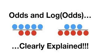
Odds and Log(Odds), Clearly Explained!!!
StatQuest with Josh Starmer
360,978 views

27:27
Linear Regression, Clearly Explained!!!
StatQuest with Josh Starmer
1,434,537 views
![Logistic Regression [Simply explained]](https://img.youtube.com/vi/C5268D9t9Ak/mqdefault.jpg)
14:22
Logistic Regression [Simply explained]
DATAtab
213,565 views

20:27
Regularization Part 1: Ridge (L2) Regression
StatQuest with Josh Starmer
1,144,390 views

14:32
SNL Weekend Update 1/4/25 | Saturday Night...
Em Vân Review
299,601 views
13:03
Statistics 101: Logistic Regression Probab...
Brandon Foltz
422,238 views

8:48
StatQuest: Logistic Regression
StatQuest with Josh Starmer
2,311,716 views

16:17
ROC and AUC, Clearly Explained!
StatQuest with Josh Starmer
1,595,580 views
1:19:34
Locally Weighted & Logistic Regression | S...
Stanford Online
616,027 views
21:58
StatQuest: Principal Component Analysis (P...
StatQuest with Josh Starmer
3,052,089 views

12:10
Mastering Odds Ratios in Logistic Regressi...
DATAtab
6,660 views

45:17
Regression Analysis | Full Course
DATAtab
865,667 views
20:47
Logistic regression with R: example
Equitable Equations
2,012 views

20:25
Logistic regression : the basics - simply ...
TileStats
38,689 views

27:27
Linear Regression, Clearly Explained!!!
StatQuest with Josh Starmer
310,919 views

16:46
Hands-On Machine Learning: Logistic Regres...
Ryan & Matt Data Science
10,349 views

12:40
Tutorial 35- Logistic Regression Indepth I...
Krish Naik
268,513 views
17:15
Logistic Regression in R, Clearly Explaine...
StatQuest with Josh Starmer
530,969 views