Nyquist Stability Criterion, Part 2

welcome back to control system lectures this is part two of our explanation of the Nyquist plot in the first part of this series I showed you the method of mapping from the S domain to the W domain using the transfer function I also explained how to use Co Xi's argument principle to our benefit what the Nyquist contour was and finally how to interpret the resulting Nyquist plot so now let me continue from there and in this video I'm going to show you a simple way to estimate a Nyquist plot by hand I'll explain how to

handle open-loop poles and zeros on the imaginary axis and then walk through an example that illustrates the power of the Nyquist plot over similar methods like the bode plot so let's get to it we'll start with estimating a Nyquist plot by hand let's say that I have this s domain transfer function 1 over s squared plus 3 s plus 2 which has these two poles s equals minus 1 and s equals minus 2 now recall from part 1 that I need to map the Nyquist contour to some other plane that I've arbitrarily called the W

plane using this transfer function so how do we do that well the most straightforward if not silly way is to take a point in the S plane on the contour and plug it into the transfer function and then plot the resulting complex number in the W plane just like I'm doing here in this example where this one point in the S plane maps to this other point in the W plane and we can continue this for every single point around the entire Nyquist contour but I'm sure you can see a problem with this not only

is this a very math intensive way but it also causes us to miss out on some very important intuition about how the Nyquist contour relates to the Nyquist plot so let me illustrate a better way to plot this first we're going to divide the Nyquist contour up into two pieces and then we'll address both piece separately the first piece can be represented by J Omega since it's just the entire J Omega line where Omega goes from negative infinity to positive infinity and we can map this entire segment all at once by plugging in J Omega

for s in our Tran for function and then sweep through all Omega by plotting the resulting real and imaginary components also because of symmetry of the poles and zeros about the real line the negative portion of the J Omega line is just the reflection of the positive portion and so we really only need to calculate the positive frequencies but I'm going to explain more about this later the second piece starts at infinity on the imaginary axis loops around to infinity on the real axis and then finally negative infinity on the imaginary axis again now I

think this segment is pretty interesting because despite the fact that it is infinitely long the entire segment maps into a single point in the W plane pretty crazy huh but there is a catch it maps to a single point only if the denominator of your transfer function is higher order than the numerator and this is called a strictly proper transfer function or if it's equal order to the numerator and this is called a proper transfer function if the numerator is of higher order than the denominator then this is not a proper transfer function and the

second segment maps to a single point for only the first two and not the last but that's okay because all physically realizable systems are either proper transfer functions or strictly proper and that's why I'm going to focus on them in this video you can show mathematically why that second segment maps into a single point in the W plane and there's a lot of great videos that do that so instead I'm going to quickly explain in a graphical sense why this is true remember from part one that the phase in the W plane is just the

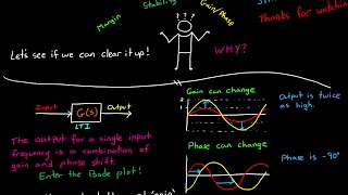
sum of the angles of the zero phasers minus the sum of the angles of the pole phasers and then for the game I didn't cover that really very well in the first video because it's a bit misleading graphically but for our following example it's acceptable to say that the gain is proportional to the magnitude of the zero phasers divided by the magnitude of the pole phasers so we're going to use that definition going forward let's take the case where there are more poles than zeros or a strictly proper system it's easy to see that if

you pick a point way out infinity since the pole phasers outnumber the zero phasers the gain will become a very large number in the numerator for the zeroes divided by more very large numbers in the denominator for the poles and that's going to put the gain really really close to zero and it's going to reach zero as that point goes out actually out to infinity and since the gain is zero we don't need to worry about the phase because the point is always at the origin in the W plane and phase would just be akin

to spinning your pencil in place at the origin it's still the same point and so we don't really have to worry about it for proper transfer functions where you have the order of the numerator and denominator equal you have this situation now along this infinity line we get a very large number from the zero divided by pretty much that exact same large number as you approach infinity this puts the gain at 1 which remember I said was just proportional to the real game so all I can say graphically is that the gain is a nonzero

but finite value so somewhere out here but what about the phase because it could exist anywhere on this circle so now phase is important well the angle for both of these phasers approach the exact same value as s goes to infinity so when you subtract the pole angle from the zero angle you always get zero degrees which means that this entire line maps to a single nonzero point on the real axis so it maps to zero for strictly proper systems and a non zero but positive real number for non strictly proper systems now to simplify

the Nyquist contour since the second segment of the Nyquist contour all mapped to the same point the W domain then we don't need to worry about it when we're plotting the point is taken care of with the positive infinity in the J Omega axis and because of the reflection we don't need the negative omegas so we really only need to plot the positive J Omega part now at the risk of confusing you I want to explain what happens if you don't have a proper transfer function in this situation on the Infinity portion of the Nyquist

contour the gain also goes to infinity since you have more zeroes than polls and as you loop around that portion of the contour the phase is also changing as you do that so in this case the portion of the Nyquist contour doesn't all map to a single point however this is really only a concern to mathematicians and not engineers since engineers deal with physically realizable systems but keep this in mind in case you come across a non proper transfer function someday so after all of that let's go through the steps to generate a Nyquist plot

first replace s by J Omega and your transfer function second sweep Omega from 0 to infinity and plot the resulting complex numbers in the W plane and then finally without picking up your pencil draw the reflection about the real axis to account for the negative omegas and don't forget to keep in mind the direction of the contour remember from part one that we trace the Nyquist contour in the clockwise direction so if we start at Omega equals zero then we trace up to Omega equals infinity and then continue around in the clockwise direction from there

I know what you're thinking I've been rambling on for eight minutes and I haven't actually told you anything about how to plot all I've done is explain why we only need to worry about plotting the positive J Omega section of the Nyquist contour rather than the whole thing but how do we estimate the plot after we replace s by J Omega well the way I prefer is actually explained very well by Professor Gopal at the Indian Institute of Technology he has a great YouTube video on it and I've placed a link in the description if

you'd like to watch the technique being explained from a professional professor but I'm going to summarize it here for simple transfer functions there are only four points that you need to solve for and then from there you can deduce the shape of the entire plot the first point is when Omega equals zero the second point is when Omega equals infinity these determine the starting and midpoint of the Nyquist plot in the W plane the third point is where the plot crosses the imaginary axis and the fourth point is where the plot crosses the real axis

so let's try this with our original transfer function and see what we get for the first point where Omega equals zero we can basically just plug in zero for each of the esses and we're going to get one half for our starting point for omega equals infinity we just plug in infinity for each of the esses and we're going to get one over a really large number which is zero which is what we expected since this is a strictly proper transfer function so the midpoint is at the origin the third and fourth points are slightly

more involved but you can solve for them by setting s equals J Omega in the transfer function and then separating out the real and imaginary components I've done that very thing here albeit really quickly at this point to solve for the imaginary intercept set the real part to 0 and then solve for Omega then plug that Omega into the imaginary part and solve for the value and that's where it crosses the imaginary axis it's a similar story to get the real intercept but this time you set the imaginary component to 0 and solve for Omega

in this case it's only 0 when Omega equals 0 or Omega equals infinity and since we've already plotted both of those points in step one and two there's really nothing else to plot it only crosses the real line at the beginning and at the mid point so now that we have this information what does it tell us well we can start with our pencil at the starting point and trace through the imaginary crossover and then through the real crossover if there is one and then end at the mid point and then we can continue on

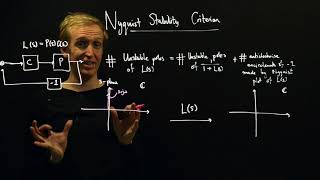
by reflecting this about the real line and we would have an approximate drawing of the Nyquist plot and from this plot we can see that the closed loop system is stable says remember there were no open-loop poles in the right-half plane and there are no encirclement of minus 1 of course this method doesn't tell us whether the plot looks like this or this but it does help us to determine closed-loop stability I'm going to plot this in MATLAB and see how close we got the first thing I'm going to do is set our systems transfer

function and then I'll plot the Nyquist plot and here it is and we did all right it doesn't look exactly the same but you can see that it starts at point five on the real axis loop down crosses over the imaginary axis and then ends at the origin and the system is stable like we predicted now a more complex transfer function is difficult to do in this method because you'll have several imaginary and real crossings but if you're trying to assess a complex transfer function you'd be better off using a computer to drive it rather

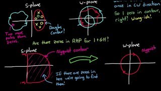
than estimate it by hand I'm going to show you an example of this at the end of this video so now the question becomes what happens if you have an open-loop pole on the imaginary axis well let's start with a single pole at the origin one over s I'll draw the Nyquist contour and pick a point to analyze somewhere up here and we're going to do a thought experiment what if we bring this point on our contour closer and closer to the pole what happens well the phase stays the same at 90 degrees but the

magnitude of the phasor gets smaller and smaller and since we're dividing by a smaller and smaller number the magnitude and the W plane tends towards infinity and once we're right on top of the pole the gain goes towards infinity since we're essentially dividing by zero the length of the phasor and the phase becomes what well it's undefined it's sort of all angles at once and yet no angle at all there is no phase since this phasor basically disappears when the point is on top of the pole in the W plane we basically have a point

that lies out at infinity but with some undefined phase so we're out of luck with understanding what that means we can't use our original Nyquist contour with poles on the imaginary axis so what do we do the solution I think is ingenious let me zoom in on the pole here so you can understand what we do we know that the contour can't lie directly on the pole otherwise the solution is undefined so why not move the contour over slightly just in that one spot since we just moved in an infinitesimal amount we've accomplished two things

the first is that we're still guaranteeing that we haven't accidentally led another closeby pole escape the contour and the second thing is that we no longer have this indeterminate solution the gain stays at infinity since we're dividing by a really small number still but the phase for our phaser very clearly starts at minus 90 degrees and loops around to plus 90 degrees so now we can draw the Nyquist plot for this system when we started Omega equals zero you can see visually that the gain is infinity since the length of the phaser is zero and

the phase is zero degrees and then as we loop around the pole the gain stays at infinity but the phase in the W plane sweeps down to minus 90 then as the contour continues up the J Omega axis the gain in the W plane goes to zero since the length of the phaser goes to infinity and finally we can complete the Nyquist plot by just drawing the reflection about the real axis and we can say that the closed loop system is stable because there are no open-loop poles in the right-half plane and no encirclements of

minus one but since you now understand the Nyquist criterion pretty well you can easily see that this adjustment to the Nyquist contour works by expanding it in the other direction also if we move it slightly to the left instead of to the right the gain is still infinity but now the phase starts at minus 180 degrees and then just like before loops down to minus 90 degrees phase then up to the origin and then finally reflected about the real axis and even though this Nyquist plot looks different than the one we drew before we can

still say that the system is stable because we have one open-loop pole in the right half plane or inside our contour and one counterclockwise encirclement of minus one therefore zero closed-loop poles in the right half plane both methods work as long as you keep track of it it's pretty awesome huh so what about an open-loop zero on the imaginary axis well you don't really have to worry about that because even though the phasor is still undefined in phase it turns out that we don't really care because the gain is zero and like I said before

when gain is zero the point lies at the origin in the W plane and so the phase doesn't really change that you can do the loop around thing like we did before but you're going to find you're going to get the exact same answer as not doing it so for open-loop zeroes perceived as normal and for open-loop poles on the imaginary axis do this fancy adjusting of the contour let me show you what happens in that when you try to plot the Nyquist plot for a system with open-loop poles on the imaginary axis you get

this vertical line but you can see that MATLAB doesn't really know how to handle plotting infinity so it just doesn't even try in order to determine stability you have to mentally complete the plot swiping either clockwise or counterclockwise at infinity and this can be tough to visualize but luckily even though MATLAB can't plot it well it will still tell you if the closed-loop system is stable and in addition to that there's this awesome plotting tool by Trond Anderson called Naik log M his script will handle infinity very nicely plus it tells you the closed-loop stability

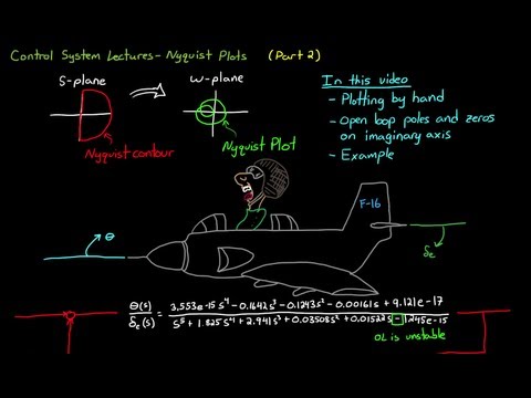
and other bits of information you can find this script at MathWorks his website and i've also included a link in the description if you'd like to download it so for this final example let me show you where the Nyquist plot really shines and that is when the open loop plant has either poles or zeros in the right half plane fighter jets are required to maneuver very quickly this gives them the edge and dogfights but a really stable airplane doesn't want to turn very quickly therefore engineers have found the best way to accomplish this is by

making the open-loop airplane slightly unstable or making it want to turn and pitch on its own and then stabilizing it using fly-by-wire feedback control the unstable plant for the pitch system of an f-16 fighter is the following where the input is the angle of the elevator and the output is the pitch angle of the aircraft now you've been tasked with designing a pitch tracking autopilot system for the f-16 you want to see if unity-feedback alone is capable of stabilizing the system you can tell that the open-loop system is unstable just by inspection by looking to

see that there is a negative in the characteristic equation but I can use MATLAB to see where the open-loop poles are for this system and that's by finding the roots of the characteristic equation and you can see that there's one just barely in the right half plane like we suspected so the open-loop system is unstable let me first plot the bode plot of this system and see what closed-loop stability information we can get from it and it's a bit hard to read even if I show stability margins in the normal sense you can't easily tell

if the closed-loop system is stable or not and in some open loop unstable cases you can't tell at all therefore in this situation you'd be safer just to plot the Nyquist plot instead and if we do this you can see very easily that there are two clockwise encirclements of minus one and since there's one open loop unstable pole this means that there is a total of three closed-loop unstable poles now with unity feedback so that's not a great design so a little bit more work needs to be done but we were able to see that

very clearly using the Nyquist plot all right well that's all I want to cover for now I hope you're starting to see the benefit of Nyquist plots and hopefully they aren't as impossible to understand as you might have previously thought in future videos I'll cover gain and phase margins with Nyquist bode and the root locus methods don't forget to subscribe so you don't miss any future videos and thanks for watching