But what is the Fourier Transform? A visual introduction.
10.39M views3756 WordsCopy TextShare

3Blue1Brown
An animated introduction to the Fourier Transform.
Help fund future projects: https://www.patreon.co...
Video Transcript:
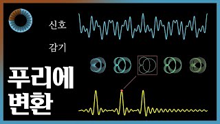
This right here is what we're going to build to this video, a certain animated approach to thinking about a super important idea from math, the Fourier transform. For anyone unfamiliar with what that is, my number one goal here is just for the video to be an introduction to that topic. But even for those of you who are already familiar with it, I still think that there's something fun and enriching about seeing what all of its components actually look like.
The central example to start is going to be the classic one, decomposing frequencies from sound. But after that I also want to show a glimpse of how this idea extends well beyond sound and frequency into many seemingly disparate areas of math, and even physics. Really, it's crazy just how ubiquitous this idea is.
Let's dive in. This sound right here is a pure A, 440 beats per second, meaning if you were to measure the air pressure right next to your headphones or your speaker as a function of time, it would oscillate up and down around its usual equilibrium in this wave, making 440 oscillations each second. A lower pitch note, like a D, has the same structure, just fewer beats per second.
And when both of them are played at once, what do you think the resulting pressure vs. time graph looks like? Well, at any point in time, this pressure difference is going to be the sum of what it would be for each of those notes individually, which let's face it is kind of a complicated thing to think about.
At some points the peaks match up with each other, resulting in a really high pressure. At other points they tend to cancel out. And all in all, what you get is a wave-ish pressure vs.
time graph that is not a pure sine wave, it's something more complicated. And as you add in other notes, the wave gets more and more complicated. But right now, all it is is a combination of four pure frequencies, so it seems needlessly complicated given the low amount of information put into it.
A microphone recording any sound just picks up on the air pressure at many different points in time, it only sees the final sum. So our central question is going to be how you can take a signal like this and decompose it into the pure frequencies that make it up. Pretty interesting, right?
Adding up those signals really mixes them all together, so pulling them back apart feels akin to unmixing multiple paint colors that have all been stirred up together. The general strategy is going to be to build for ourselves a mathematical machine that treats signals with a given frequency differently from how it treats other signals. To start, consider simply taking a pure signal, say with a lowly 3 beats per second, so we can plot it easily.
And let's limit ourselves to looking at a finite portion of this graph, in this case the portion between 0 seconds and 4. 5 seconds. The key idea is going to be to take this graph and sort of wrap it up around a circle.
Concretely, here's what I mean by that. Imagine a little rotating vector where at each point in time its length is equal to the height of our graph for that time. So high points of the graph correspond to a greater distance from the origin, and low points end up closer to the origin.
And right now I'm drawing it in such a way that moving forward 2 seconds in time corresponds to a single rotation around the circle. Our little vector drawing this wound up graph is rotating at half a cycle per second. So this is important, there are two different frequencies at play here.
There's the frequency of our signal, which goes up and down 3 times per second, and then separately there's the frequency with which we're wrapping the graph around the circle, which at the moment is half of a rotation per second. But we can adjust that second frequency however we want. Maybe we want to wrap it around faster?
Or maybe we go and wrap it around slower? And that choice of winding frequency determines what the wound up graph looks like. Some of the diagrams that come out of this can be pretty complicated, although they are very pretty, but it's important to keep in mind that all that's happening here is that we're wrapping the signal around a circle.
The vertical lines that I'm drawing up top, by the way, are just a way to keep track of the distance on the original graph that corresponds to a full rotation around the circle. So lines spaced out by 1. 5 seconds would mean it takes 1.
5 seconds to make one full revolution. And at this point we might have some sort of vague sense that something special will happen when the winding frequency matches the frequency of our signal, 3 beats per second. All of the high points on the graph happen on the right side of the circle, and all of the low points happen on the left.
But how precisely can we take advantage of that in our attempt to build a frequency unmixing machine? Well, imagine this graph is having some kind of mass to it, like a metal wire. This little dot is going to represent the center of mass of that wire.
As we change the frequency and the graph winds up differently, that center of mass kind of wobbles around a bit. And for most of the winding frequencies, the peaks and valleys are all spaced out around the circle in such a way that the center of mass stays pretty close to the origin. But when the winding frequency is the same as the frequency of our signal, in this case 3 cycles per second, all of the peaks are on the right, and all of the valleys are on the left, so the center of mass is unusually far to the right.
Here, to capture this, let's draw some kind of plot that keeps track of where that center of mass is for each winding frequency. Of course, the center of mass is a two-dimensional thing, it requires two coordinates to fully keep track of, but for the moment, let's only keep track of the x-coordinate. So for a frequency of zero, when everything is bunched up on the right, this x-coordinate is relatively high.
And then as you increase that winding frequency, and the graph balances out around the circle, the x-coordinate of that center of mass goes closer to zero, and it just kind of wobbles around a bit. But then, at 3 beats per second, there's a spike, as everything lines up to the right. This right here is the central construct, so let's sum up what we have so far.
We have that original intensity vs time graph, and then we have the wound up version of that in some two-dimensional plane, and then as a third thing, we have a plot for how the winding frequency influences the center of mass of that graph. And by the way, let's look back at those really low frequencies near zero. This big spike around zero in our new frequency plot just corresponds to the fact that the whole cosine wave is shifted up.
If I had chosen a signal that oscillates around zero, dipping into negative values, then as we play around with various winding frequencies, this plot of the winding frequency vs center of mass would only have a spike at the value of 3. But negative values are a little bit weird and messy to think about, especially for a first example, so let's just continue thinking in terms of the shifted up graph. I just want you to understand that that spike around zero only corresponds to the shift.
Our main focus, as far as frequency decomposition is concerned, is that bump at 3. This whole plot is what I'll call the almost Fourier transform of the original signal. There's a couple small distinctions between this and the actual Fourier transform, which I'll get to in a couple minutes, but already you might be able to see how this machine lets us pick out the frequency of a signal.
Just to play around with it a little bit more, take a different Fourier signal, let's say with a lower frequency of 2 beats per second, and do the same thing. Wind it around a circle, imagine different potential winding frequencies, and as you do that keep track of where the center of mass of that graph is, and then plot the x coordinate of that center of mass as you adjust the winding frequency. Just like before, we get a spike when the winding frequency is the same as the signal frequency, which in this case is when it equals 2 cycles per second.
But the real key point, the thing that makes this machine so delightful, is how it enables us to take a signal consisting of multiple frequencies and pick out what they are. Imagine taking the two signals we just looked at, the wave with 3 beats per second and the wave with 2 beats per second, and add them up. Like I said earlier, what you get is no longer a nice pure cosine wave, it's something a little more complicated.
But imagine throwing this into our winding frequency machine. It is certainly the case that as you wrap this thing around it looks a lot more complicated, you have this chaos and chaos and chaos and chaos, and then whoop, things seem to line up really nicely at 2 cycles per second. Then as you continue on it's more chaos and more chaos and more chaos and chaos and chaos and chaos, whoop, things nicely align again at 3 cycles per second.
And like I said before, the wound up graph can look kind of busy and complicated, but all it is is the relatively simple idea of wrapping the graph around a circle. It's just a more complicated graph and a pretty quick winding frequency. Now what's going on here with the two different spikes is that if you were to take two signals and then apply this almost Fourier transform to each of them individually, and then add up the results, what you get is the same as if you first added up the signals and then applied this almost Fourier transform.
And the attentive viewers among you might want to pause and ponder and convince yourself that what I just said is actually true. It's a pretty good test to verify for yourself that it's clear what exactly is being measured inside this winding machine. Now this property makes things really useful to us, because the transform of a pure frequency is close to zero everywhere except for a spike around that frequency, so when you add together two pure frequencies, the transform graph just has these little peaks above the frequencies that went into it.
So this little mathematical machine does exactly what we wanted. It pulls out the original frequencies from their jumbled up sums, unmixing the mixed bucket of paint. And before continuing into the full math that describes this operation, let's just get a quick glimpse of one context where this thing is useful, sound editing.
Let's say that you have some recording and it's got an annoying high pitch that you would like to filter out. Well at first your signal is coming in as a function of various intensities over time, different voltages given to your speaker from one millisecond to the next. But we want to think of this in terms of frequencies.
So when you take the Fourier transform of that signal, the annoying high pitch is going to show up just as a spike at some high frequency. Filtering that out by just smushing the spike down, what you'd be looking at is the Fourier transform of a sound that's just like your recording, only without that high frequency. Luckily there's a notion of an inverse Fourier transform that tells you which signal would have produced this as its Fourier transform.
I'll be talking about that inverse much more fully in the next video, but long story short, applying the Fourier transform to the Fourier transform gives you back something close to the original function. Kind of, this is a little bit of a lie, but it's in the direction of truth. And most of the reason it's a lie is that I still have yet to tell you what the actual Fourier transform is, since it's a little more complex than this x-coordinate of the center of mass idea.
First off, bringing back this wound up graph and looking at its center of mass, the x-coordinate is really only half the story, right? I mean, this thing is in two dimensions, it's got a y-coordinate as well. And as is typical in math, whenever you're dealing with something two-dimensional, it's elegant to think of it as the complex plane, where this center of mass is going to be a complex number that has both a real and an imaginary part.
And the reason for talking in terms of complex numbers, rather than just saying it has two coordinates, is that complex numbers lend themselves to really nice descriptions of things that have to do with winding and rotation. For example, Euler's formula famously tells us that if you take e to some number times i, you're going to land on the point that you get if you were to walk that number of units around a circle with radius 1 counterclockwise starting on the right. So imagine you wanted to describe rotating at a rate of 1 cycle per second.
One thing you could do is take the expression e to the 2 pi times i times t, where t is the amount of time that has passed, since for a circle with radius 1, 2 pi describes the full length of its circumference. And this is a little dizzying to look at, so maybe you want to describe a different frequency, something lower and more reasonable, and for that you would just multiply that time t in the exponent by the frequency f. For example, if f was 1 tenth, then this vector makes one full turn every 10 seconds, since the time t has to increase all the way to 10 before the full exponent looks like 2 pi i.
I have another video giving some intuition on why this is the behavior of e to the x for imaginary inputs, if you're curious, but for right now we're just going to take it as a given. Now why am I telling you this, you might ask? Well it gives us a really nice way to write down the idea of winding up the graph into a single tight little formula.
First off, the convention in the context of Fourier transforms is to think about rotating in the clockwise direction, so let's throw a negative sign up into that exponent. Now take some function describing a signal intensity versus time, like this pure cosine wave we had before, and call it g of t. If you multiply this exponential expression times g of t, it means that the rotating complex number is getting scaled up and down according to the value of this function.
So you can think of this little rotating vector with its changing length as drawing the wound up graph. So think about it, this is awesome, this really small expression is a super elegant way to encapsulate the whole idea of winding a graph around a circle with a variable frequency, f. And remember, the thing we want to do with this wound up graph is to track its center of mass, so think about what formula is going to capture that.
Well, to approximate it at least, you might sample a whole bunch of times from the original signal, see where those points end up on the wound up graph, and then just take an average, that is, add them all together as complex numbers, and then divide by the number of points you've sampled. This will become more accurate if you sample more points which are closer together. And in the limit, rather than looking at the sum of a whole bunch of points divided by the number of points, you take an integral of this function divided by the size of the time interval we're looking at.
The idea of integrating a complex valued function might seem weird, and to anyone who's shaky with calculus maybe even intimidating, but the underlying meaning here really doesn't require any calculus knowledge. The whole expression is just the center of mass of the wound up graph. So great, step by step, we have built up this kind of complicated but let's face it, surprisingly small expression for the whole winding machine idea I talked about, and now there is only one final distinction to point out between this and the actual honest-to-goodness Fourier transform, namely, just don't divide out by the time interval.
The Fourier transform is just the integral part of this. What that means is that instead of looking at the center of mass, you would scale it up by some amount. If the portion of the original graph you were using spanned 3 seconds, you would multiply the center of mass by 3.
If it was spanning 6 seconds, you would multiply the center of mass by 6. Physically, this has the effect that when a certain frequency persists for a long time, then the magnitude of the Fourier transform at that frequency is scaled up more and more. For example, what we're looking at here is how when you have a pure frequency of 2 beats per second and you wind it around the graph at 2 cycles per second, the center of mass stays in the same spot, just tracing out the same shape.
But the longer that signal persists, the larger the value of the Fourier transform at that frequency. For other frequencies, even if you just increase it by a bit, this is cancelled out by the fact that for longer time intervals, you're giving the wound-up graph more of a chance to balance itself around the circle. That is a lot of different moving parts, so let's step back and summarize what we have so far.
The Fourier transform of an intensity vs. time function, like g of t, is a new function, which doesn't have time as an input, but instead takes in a frequency, what I've been calling the winding frequency. In terms of notation, by the way, the common convention is to call this new function g-hat with a little circumflex on top of it.
The output of this function is a complex number, some point in the 2d plane that corresponds to the strength of a given frequency in the original signal. The plot I've been graphing for the Fourier transform is just the real component of that output, the x-coordinate, but you could also graph the imaginary component separately if you wanted a fuller description. And all of this is encapsulated inside that formula we built up.
And out of context, you can imagine how seeing this formula would seem sort of daunting, but if you understand how exponentials correspond to rotation, how multiplying that by the function g of t means drawing a wound up version of the graph, and how an integral of a complex valued function can be interpreted in terms of a center of mass idea, you can see how this whole thing carries with it a very rich intuitive meaning. And by the way, one quick small note before we can call this wrapped up. Even though in practice, with things like sound editing, you'll be integrating over a finite time interval, the theory of Fourier transforms is often phrased where the bounds of this integral are negative infinity and infinity.
Concretely, what that means is that you consider this expression for all possible finite time intervals, and you just ask, what is its limit as that time interval grows to infinity? And man oh man, there is so much more to say. So much, I don't want to call it done here.
This transform extends to corners of math well beyond the idea of extracting frequencies from signal. So the next video I put out is going to go through a couple of these, and that's really where things start getting interesting. So stay subscribed for when that comes out, or an alternate option is to just binge on a couple 3Blue and Brown videos so that the YouTube recommender is more inclined to show you new things that come out.
Really the choice is yours. And to close things off, I have something pretty fun, a mathematical puzzler from this video's sponsor, Jane Street, who's looking to recruit more technical talent. So let's say that you have a closed bounded convex set C sitting in 3D space, and then let B be the boundary of that space, the surface of your complex blob.
Now imagine taking every possible pair of points on that surface and adding them up, doing a vector sum. Let's name this set of all possible sums D. Your task is to prove that D is also a convex set.
So Jane Street is a quantitative trading firm, and if you're the kind of person who enjoys math and solving puzzles like this, the team there really values intellectual curiosity, so they might be interested in hiring you. And they're looking both for full-time employees and interns. For my part, I can say the couple of people I've interacted with there just seem to love math and sharing math, and when they're hiring, they look less at a background in finance than they do at how you think, how you learn, and how you solve problems, hence the sponsorship of a 3Blue1Brown video.
If you want the answer to that puzzler, or to learn more about what they do, or to apply for open positions, go to janestreet. com slash 3b1b. Thank you.
Related Videos
19:21
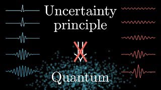
The more general uncertainty principle, re...
3Blue1Brown
2,029,441 views
24:47
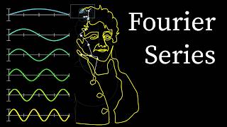
But what is a Fourier series? From heat f...
3Blue1Brown
17,841,329 views

28:23
The Fast Fourier Transform (FFT): Most Ing...
Reducible
1,894,315 views
18:39
This equation will change how you see the ...
Veritasium
16,043,277 views

14:48
The Fourier Series and Fourier Transform D...
Up and Atom
812,170 views

23:01
But what is a convolution?
3Blue1Brown
2,644,826 views

43:31
Coding Adventure: Sound (and the Fourier T...
Sebastian Lague
360,115 views
![The most beautiful equation in math, explained visually [Euler’s Formula]](https://img.youtube.com/vi/f8CXG7dS-D0/mqdefault.jpg)
26:57
The most beautiful equation in math, expla...
Welch Labs
697,501 views

57:24
Terence Tao at IMO 2024: AI and Mathematics
AIMO Prize
295,784 views
15:46
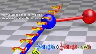
Fourier Transform, Fourier Series, and fre...
Physics Videos by Eugene Khutoryansky
3,164,668 views

22:56
Visualizing 4D Pt.1
HyperCubist Math
489,672 views

18:00
The intuition behind Fourier and Laplace t...
Zach Star
1,022,389 views

34:29
Wavelets: a mathematical microscope
Artem Kirsanov
627,414 views

40:06
A tale of two problem solvers (Average cub...
3Blue1Brown
2,743,685 views
19:43
푸리에 변환이 뭐냐면... 그려서 보여드리겠습니다.
3Blue1Brown 한국어
422,535 views
30:17
This Is the Calculus They Won't Teach You
A Well-Rested Dog
3,215,413 views
19:20
Understanding the Discrete Fourier Transfo...
MATLAB
161,053 views

16:17
The Revolutionary Genius Of Joseph Fourier
Dr. Will Wood
146,602 views
21:29
Are solid objects really “solid”?
AlphaPhoenix
5,720,818 views

22:11
But what is the Riemann zeta function? Vis...
3Blue1Brown
4,706,721 views