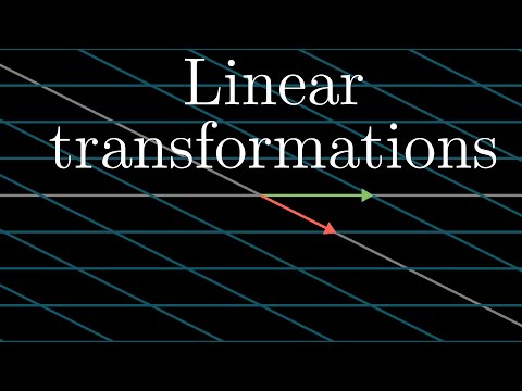
Linear transformations and matrices | Chapter 3, Essence of linear algebra
5.22M views1810 WordsCopy TextShare
3Blue1Brown
Quite possibly the most important idea for understanding linear algebra.
Help fund future projects: ...
Video Transcript:
Hey everyone! If I had to choose just one topic that makes all of the others in linear algebra start to click, and which too often goes unlearned the first time a student takes linear algebra, it would be this one. The idea of a linear transformation and its relation to matrices.
For this video, I'm just going to focus on what these transformations look like in the case of two dimensions, and how they relate to the idea of matrix vector multiplication. In particular, I want to show you a way to think about matrix vector multiplication that doesn't rely on memorization. To start, let's just parse this term, linear transformation.
Transformation is essentially a fancy word for function. It's something that takes in inputs and spits out an output for each one. Specifically, in the context of linear algebra, we like to think about transformations that take in some vector and spit out another vector.
So why use the word transformation instead of function if they mean the same thing? Well, it's to be suggestive of a certain way to visualize this input-output relation. You see, a great way to understand functions of vectors is to use movement.
If a transformation takes some input vector to some output vector, we imagine that input vector moving over to the output vector. Then to understand the transformation as a whole, we might imagine watching every possible input vector move over to its corresponding output vector. It gets really crowded to think about all of the vectors all at once, each one as an arrow.
So as I mentioned last video, a nice trick is to conceptualize each vector not as an arrow, but as a single point, the point where its tip sits. That way, to think about a transformation taking every possible input vector to some output vector, we watch every point in space moving to some other point. In the case of transformations in two dimensions, to get a better feel for the whole shape of the transformation, I like to do this with all of the points on an infinite grid.
I also sometimes like to keep a copy of the grid in the background, just to help keep track of where everything ends up relative to where it starts. The effect for various transformations moving around all of the points in space is, you've got to admit, beautiful. It gives the feeling of squishing and morphing space itself.
As you can imagine though, arbitrary transformations can look pretty complicated. But luckily, linear algebra limits itself to a special type of transformation, ones that are easier to understand, called linear transformations. Visually speaking, a transformation is linear if it has two properties.
All lines must remain lines without getting curved, and the origin must remain fixed in place. For example, this right here would not be a linear transformation, since the lines get all curvy. And this one right here, although it keeps the lines straight, is not a linear transformation, because it moves the origin.
This one here fixes the origin, and it might look like it keeps lines straight, but that's just because I'm only showing the horizontal and vertical grid lines. When you see what it does to a diagonal line, it becomes clear that it's not at all linear, since it turns that line all curvy. In general, you should think of linear transformations as keeping grid lines parallel and evenly spaced.
Some linear transformations are simple to think about, like rotations about the origin. Others are a little trickier to describe with words. So, how do you think you could describe these transformations numerically?
If you were, say, programming some animations to make a video teaching the topic, what formula do you give the computer so that if you give it the coordinates of a vector, it can give you the coordinates of where that vector lands? It turns out that you only need to record where the two basis vectors, i-hat and j-hat, each land, and everything else will follow from that. For example, consider the vector v with coordinates negative 1, 2, meaning that it equals negative 1 times i-hat plus 2 times j-hat.
If we play some transformation and follow where all three of these vectors go, the property that grid lines remain parallel and evenly spaced has a really important consequence. The place where v lands will be negative 1 times the vector where i-hat landed plus 2 times the vector where j-hat landed. In other words, it started off as a certain linear combination of i-hat and j-hat, and it ends up as that same linear combination of where those two vectors landed.
This means you can deduce where v must go based only on where i-hat and j-hat each land. This is why I like keeping a copy of the original grid in the background. For the transformation shown here, we can read off that i-hat lands on the coordinates 1, negative 2, and j-hat lands on the x-axis over at the coordinates 3, 0.
This means that the vector represented by negative 1 i-hat plus 2 times j-hat ends up at negative 1 times the vector 1, negative 2 plus 2 times the vector 3, 0. Adding that all together, you can deduce that it has to land on the vector 5, 2. This is a good point to pause and ponder, because it's pretty important.
Now, given that I'm actually showing you the full transformation, you could have just looked to see that v has the coordinates 5, 2. But the cool part here is that this gives us a technique to deduce where any vectors land so long as we have a record of where i-hat and j-hat each land without needing to watch the transformation itself. Write the vector with more general coordinates, x and y, and it will land on x times the vector where i-hat lands, 1, negative 2, plus y times the vector where j-hat lands, 3, 0.
Carrying out that sum, you see that it lands at 1x plus 3y, negative 2x plus 0y. I give you any vector, and you can tell me where that vector lands using this formula. What all of this is saying is that a two-dimensional linear transformation is completely described by just four numbers, the two coordinates for where i-hat lands and the two coordinates for where j-hat lands.
Isn't that cool? It's common to package these coordinates into a 2x2 grid of numbers called a 2x2 matrix, where you can interpret the columns as the two special vectors where i-hat and j-hat each land. If you're given a 2x2 matrix describing a linear transformation and some specific vector, and you want to know where that linear transformation takes that vector, you can take the coordinates of the vector, multiply them by the corresponding columns of the matrix, then add together what you get.
This corresponds with the idea of adding the scaled versions of our new basis vectors. Let's see what this looks like in the most general case, where your matrix has entries A, B, C, D. And remember, this matrix is just a way of packaging the information needed to describe a linear transformation.
Always remember to interpret that first column, AC, as the place where the first basis vector lands, and that second column, BD, as the place where the second basis vector lands. When we apply this transformation to some vector xy, what do you get? Well, it'll be x times AC plus y times BD.
Putting this together, you get a vector Ax plus By, Cx plus Dy. You could even define this as matrix vector multiplication, when you put the matrix on the left of the vector like it's a function. Then, you could make high schoolers memorize this without showing them the crucial part that makes it feel intuitive.
But, isn't it more fun to think about these columns as the transformed versions of your basis vectors, and to think about the result as the appropriate linear combination of those vectors? Let's practice describing a few linear transformations with matrices. For example, if we rotate all of space 90 degrees counterclockwise, then i-hat lands on the coordinates 0, 1.
And j-hat lands on the coordinates negative 1, 0. So the matrix we end up with has columns 0, 1, negative 1, 0. To figure out what happens to any vector after a 90-degree rotation, you could just multiply its coordinates by this matrix.
Here's a fun transformation with a special name, called a shear. In it, i-hat remains fixed, so the first column of the matrix is 1, 0. But j-hat moves over to the coordinates 1, 1, which become the second column of the matrix.
And at the risk of being redundant here, figuring out how a shear transforms a given vector comes down to multiplying this matrix by that vector. Let's say we want to go the other way around, starting with a matrix, say with columns 1, 2 and 3, 1, and we want to deduce what its transformation looks like. Pause and take a moment to see if you can imagine it.
One way to do this is to first move i-hat to 1, 2, then move j-hat to 3, 1. Always moving the rest of space in such a way that keeps gridlines parallel and evenly spaced. If the vectors that i-hat and j-hat land on are linearly dependent, which, if you recall from last video, means that one is a scaled version of the other, it means that the linear transformation squishes all of 2D space onto the line where those two vectors sit, also known as the one-dimensional span of those two linearly dependent vectors.
To sum up, linear transformations are a way to move around space such that gridlines remain parallel and evenly spaced, and such that the origin remains fixed. Delightfully, these transformations can be described using only a handful of numbers, the coordinates of where each basis vector lands. Matrices give us a language to describe these transformations, where the columns represent those coordinates, and matrix-vector multiplication is just a way to compute what that transformation does to a given vector.
The important takeaway here is that every time you see a matrix, you can interpret it as a certain transformation of space. Once you really digest this idea, you're in a great position to understand linear algebra deeply. Almost all of the topics coming up, from matrix multiplication to determinants, change of basis, eigenvalues, all of these will become easier to understand once you start thinking about matrices as transformations of space.
Most immediately, in the next video, I'll be talking about multiplying two matrices together. See you then! Thank you for watching!
Related Videos
10:04
Matrix multiplication as composition | Cha...
3Blue1Brown
3,272,630 views

46:24
How are holograms possible?
3Blue1Brown
496,777 views

12:09
Inverse matrices, column space and null sp...
3Blue1Brown
2,903,692 views

25:41
The deeper meaning of matrix transpose
Mathemaniac
378,068 views
13:52
Linear transformations | Matrix transforma...
Khan Academy
1,643,775 views

9:59
Linear combinations, span, and basis vecto...
3Blue1Brown
5,471,867 views
17:16
Eigenvectors and eigenvalues | Chapter 14,...
3Blue1Brown
4,880,476 views

16:26
Dear linear algebra students, This is what...
Zach Star
1,149,628 views
30:17
This Is the Calculus They Won't Teach You
A Well-Rested Dog
3,300,210 views

14:20
ALL OF PHYSICS explained in 14 Minutes
Wacky Science
3,127,966 views
22:09
The Simplest Math Problem No One Can Solve...
Veritasium
41,206,083 views
27:07
How (and why) to raise e to the power of a...
3Blue1Brown
2,866,936 views
49:27
30. Linear Transformations and Their Matrices
MIT OpenCourseWare
436,739 views

9:52
Vectors | Chapter 1, Essence of linear alg...
3Blue1Brown
8,678,108 views

10:03
The determinant | Chapter 6, Essence of li...
3Blue1Brown
3,842,305 views

1:02:46
Grant Sanderson: 3Blue1Brown and the Beaut...
Lex Fridman
553,285 views
17:05
The essence of calculus
3Blue1Brown
9,328,214 views

23:29
How Imaginary Numbers Were Invented
Veritasium
18,065,256 views
14:12
Dot products and duality | Chapter 9, Esse...
3Blue1Brown
2,557,043 views