Locally Weighted & Logistic Regression | Stanford CS229: Machine Learning - Lecture 3 (Autumn 2018)

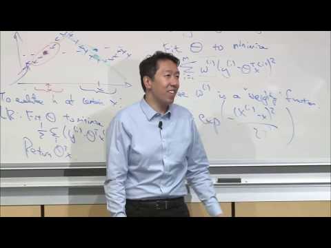
What I'd like to do today is continue our discussion of supervised learning. So last Wednesday, you saw the linear regression algorithm, uh, including both gradient descent, how to formulate the problem, then gradient descent, and then the normal equations. What I'd like to do today is, um, talk about locally weighted regression which is a, a way to modify linear regressions and make it fit very non-linear functions so you aren't just fitting straight lines. And then I'll talk about a probabilistic interpretation of linear regression and that will lead us into the first classification algorithm you see in

this class called logistic regression, and we'll talk about an algorithm called Newton's method for logistic regression. And so the dependency of ideas in this class is that, um, locally weighted regression will depend on what you learned in linear regression. And then, um, we're actually gonna just cover the key ideas of locally weighted regression, and let you play with some of the ideas yourself in the, um, problem set 1 which we'll release later this week. And then, um, I guess, give a probabilistic interpretation of linear regression, logistic regression depend on that, um, and Newton's method is

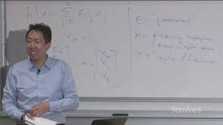
for logistic regression, okay? To recap the notation you saw on Wednesday, we use this notation x_i, i- y_i to denote a single training example where x_i was n + 1 dimensional. So if you have two features, the size of the house and the number of bedrooms, then x_i would be 2 + 1, it would 3-dimensional because we have introduced a new, uh, sort of fake feature x_0 which was always set to the value of 1. Uh, and then yi, in the case of regression is always a real number and what's the number of training examples

and what's the number of features and, uh, this was the hypothesis, right? It's a linear function of the features x, um, including this feature x_0 which is always set to 1, and, uh, j was the cost function you would minimize, you minimize this as function of j to find the parameters Theta for your straight line fit to the data, okay? So that's what you saw last Wednesday. Um, now if you have a dataset, that looks like that, where this is the size of a house and this is the price of a house. What you saw

on Wednesday- last Wednesday, was an algorithm to fit a straight line, right to this data so the hypothesis was of the form Theta 0 + Theta 1 x_0- x_0- Theta 1 x_1 to be very specific. But with this dataset maybe it actually looks, you know, maybe the data looks a little bit like that and so one question that you have to address when, uh, fitting models to data is what are the features you want? Do you want to fit a straight line to this problem or do you want to fit a hypothesis of the form,

um, Theta 1x + Theta 2x squared since this may be a quadratic function, right? Now the problem with quadratic functions is that quadratic functions eventually start, you know, curving back down so that will be a quadratic function. This arc starts curving back down. So maybe you don't want to fit a quadratic function. Uh, instead maybe you want, uh, to fit something like that. If- if housing prices sort of curved down a little bit but you don't want it to eventually curve back down the way a quadratic function would, right? Um, so- oh, and, and if

you want to do this the way you would implement is is you define the first feature x_1 = x and the second feature x_2 = x squared or you define x_1 to be equal to x and x_2 = square root of x, right and by defining a new feature x_2 which would be the square root of x and square root of x. Then the machinery that you saw from Wednesday of linear regression applies to fit these types of, um, these types of functions of the data. So later this quarter you'll hear about feature selection algorithms,

which is a type of algorithm for automatically deciding, do you want x squared as a feature or square root of x as a feature or maybe you want, um, log of x as a feature, right. But what set of features, um, does the best job fitting the data that you have if it's not fit well by a perfectly straight line. Um, what I would like to do today is- so, so you'll hear about feature selection later this quarter. What I want to share with you today is a different way of addressing this out- this problem

of whether the data isn't just fit well by a straight line and in particular I wanna share with you an idea called, uh, locally weighted regression or locally weighted linear regression. So let me use a slightly different, um, example to illustrate this. Um, which is, uh, which is that, you know, if you have a dataset that looks like that. [NOISE] So it's pretty clear what the shape of this data is. Um, but how do you fit a curve that, you know, kind of looks like that, right? And it's, it's actually quite difficult to find features,

is it square root of x, log of x, x cube, like third root of x, x the power of 2/3. But what is the set of features that lets you do this? So we'll sidestep all those problems with an algorithm called, uh, locally weighted regression. Um, okay, and to introduce a bit more machine learning terminology. Um, in machine learning we sometimes distinguish between parametric learning algorithms and non-parametric learning algorithms. But in a parametric learning algorithm does, uh, uh, you fit some fixed set of parameters such as Theta i to data and so linear regression as

you saw last Wednesday is a parametric learning algorithm because there's a fixed set of parameters, the Theta i's, so you fit to data and then you're done, right. Locally weighted regression will be our first exposure to a non-parametric learning algorithm. Um, and what that means is that the amount of data/parameters, uh, you need to keep grows and in this case it grows linearly with the size of the data, with size of training set, okay? So with the parametric learning algorithm, no matter how big your training, uh, your training set is, you fit the parameters Theta

i. Then you could erase a training set from your computer memory and make predictions just using the parameters Theta i and in a non-parametric learning algorithm which we'll see in a second, the amount of stuff you need to keep around in computer memory or the amount of stuff you need to store around grows linearly as a function of the training set size. Uh, and so this type of algorithm is your- may, may, may not be great if you have a really, really massive dataset because you need to keep all of the data around your- in

computer memory or on disk just to make predictions, okay? So- but we'll see an example of this and one of the effects of this is that with that, it'll, it'll be able to fit that data that I drew up there, uh, quite well without you needing to fiddle manually with features. Um, and again you get to practice implementing locally weighted regression in the homework. So I'm gonna go over the height of ideas relatively quickly and then let you, uh, uh, gain practice, uh, in the problem set. All right. So let me redraw that dataset, it'd

be something like this. [NOISE] All right. So- so say you have a dataset like this. Um, now for linear regression if you want to evaluate h at a certain value of the input, right? So to make a prediction at a certain value of x what you- for linear regression what you do is you fit theta, you know, to minimize this cost function. [NOISE] And then you return Theta transpose x, right? So you fit a straight line and then, you know, if you want to make a prediction at this value x you then return say the

transpose x. For locally weighted regression, um, you do something slightly different. Which is if this is the value of x and you want to make a prediction around that value of x. What you do is you look in a lo- local neighborhood at the training examples close to that point x where you want to make a prediction. And then, um, I'll describe this informally for now but we'll- we'll formalize this in math for the second. Um, but focusing mainly on these examples and, you know, looking a little bit at further all the examples. But really

focusing mainly on these examples, you try to fit a straight line like that, focusing on the training examples that are close to where you want to make a prediction. And by close I mean the values are similar, uh, on the x axis. The x values are similar. And then to actually make a prediction, you will, uh, use this green line that you just fit to make a prediction at that value of x, okay? Now if you want to make a prediction at a different point. Um, let's say that, you know, the user now says, "Hey,

make a prediction for this point." Then what you would do is you focus on this local area, kinda look at those points. Um, and when I say focus say, you know, put most of the weights on these points but you kinda take a glance at the points further away, but mostly the attention is on these for the straight line to that, and then you use that straight line to make a prediction, okay. Um, and so to formalize this in locally weighted regression, um, you will fit Theta to minimize a modified cost function [NOISE] Where wi

is a weight function. Um, and so a good- well the default choice, a common choice for wi will be this. [NOISE] Right, um, I'm gonna add something to this equation a little bit later. But, uh, wi is a weighting function where, notice that this, this formula has a defining property, right? If xi - x is small, then the weight will be close to 1. Because, uh, if xi x- so x is the location where you want to make a prediction and xi is the input x for your ith training example. So wi is a weighting

function, um, that's a value between 0 and 1 that tells you how much should you pay attention to the values of xi, yi when fitting say this green line or that red line. And so if xi - x is small so that's a training example that is close to where you want to make the prediction for x. Then this is about e to the 0, right, e to the -0 if the- if the numerator here is small and e to the 0 is close to 1. Right, um, and conversely if xi - x is large,

then wi is close to 0. And so if xi is very far away so let's see if it's fitting this green line. And this is your example, xi yi then it's saying, give this example all the way out there if you're fitting the green line where you look at this first x saying that example should have weight fairly close to 0, okay? Um, and so if you, um, look at the cost function, the main modification to the cost function we've made is that we've added this weighting term, right? And so what locally weighted regression does

is the same. If an example xi is far from where you wanna make a prediction multiply that error term by 0 or by a constant very close to 0. Um, whereas if it's close to where you wanna make a prediction multiply that error term by 1. And so the net effect of this is that this is summing if, if, you know, the terms multiplied by 0 disappear, right? So the net effect of this is that the sums over essentially only the terms, uh, for the squared error for the examples that are close to the value,

close to the value of x where you want to make a prediction, okay? Um, and that's why when you fit Theta to minimize this, you end up paying attention only to the points, only to the examples close to where you wanna make a prediction and fitting a line like a green line over there, okay? Um, so let me draw a couple more pictures to- to- to illustrate this. Um, so if- let me draw a slightly smaller data set just to make this easier to illustrate. Um, so that's your training set. So there's your examples x1,

x2, x3, x4. And if you want to make a prediction here, right, at that point x, then, um, this curve here looks the- the- the shape of this curve is actually like this, right? Um, and this is the shape of a Gaussian bell curve. But this has nothing to do with a Gaussian density, right, so this thing does not integrate to 1. So- so it's just sometimes you ask well, is this- is this using a Gaussian density? The answer is no. Uh, this is just a function that, um, is shaped a lot like a Gaussian

but, you know, Gaussian densities, probability density functions have to integrate to 1 and this does not. So there's nothing to do with a Gaussian probability density. Question? So how- how do you choose the width of the- Oh, so how do you choose the width, lemmi get back to that. Yeah. Um, and so for this example this height here says give this example a weight equal to the height of that thing. Give this example a weight to the height of this, height of this, height of that, right? Which is why if you actually- if you have

an example this way out there, you know, is given a weight that's essentially 0. Which is why it's weighting only the nearby examples when trying to fit a straight line, right, uh, for the- for making predictions close to this, okay? Um, now so one last thing that I wanna mention which is, um, the- the- the question just now which is how do you choose the width of this Gaussian density, right? How fat it is or how thin should it be? Um, and this decides how big a neighborhood should you look in order to decide what's

the neighborhood of points you should use to fit this, you know, local straight line. And so, um, for Gaussian function like this, uh, this- I'm gonna call this the, um, bandwidth parameter tau, right? And this is a parameter or a hyper-parameter of the algorithm. And, uh, depending on the choice of tau, um, uh, you can choose a fatter or a thinner bell-shaped curve, which causes you to look in a bigger or a narrower window in order to decide, um, you know, how many nearby examples to use in order to fit the straight line, okay? And

it turns out that, um, and I wanna leave- I wanna leave you to discover this yourself in the problem set. Um, if- if you've taken a little bit of machine learning elsewhere I've heard of the terms [inaudible] Test. It's on? Okay, good. It was on. Good. It turns out that, um, the choice of the bandwidth tau has an effect on, uh, overfitting and underfitting. If you don't know what those terms mean don't worry about it, we'll define them later in this course. But, uh, what you get to do in the problem set is, uh, play

with tau yourself and see why, um, if tau is too broad, you end up fitting, um, you end up over-smoothing the data and if tau is too thin you end up fitting a very jagged fit to the data. And if any of these things don't make sense yet don't worry about it they'll make sense after you play a bit in the- in the problem set, okay? Um, so yeah, since- since you- you play with the varying tau in the problem set and see for yourself the net impact of that, okay? Question? Is tau raised to

power there or is that just a- just a- [NOISE] Thank you, uh, this is tau squared. Yeah. Yeah. So- so what happens if you need to invert, uh, the [inaudible] What happens if you need to infer the value of h outside the scope of the dataset? It turns out that you can still use this algorithm. It's just that, um, its results may not be very good. Yeah. It- it- it depends I guess. Um, locally linear regression is usually not greater than extrapolation, but then most- many learning algorithms are not good at extrapolation. So all- all

the formulas still work, you can still implement this. But, um, yeah. You can also try- you can also try a linear problem set and see what happens. Yeah. One last question. Is it possible to have like a vertical tau depending on whether some parts of your data have lots of- Yeah. Yes, this is mostly for the variable tau depending- Uh, uh, yes, it is, uh, and there are quite complicated ways to choose tau based on how many points there on the local region and so on. Yes. There's a huge literature on different formulas actually for

example instead of this Gaussian bump thing, uh, there's, uh, sometimes people use that triangle shape function. So it actually goes to zero outside some small rings. So there are, there are many versions of this algorithm. Um, so I tend to use, uh, a locally weighted linear regression when, uh, you have a relatively low dimensional data set. So when the number of features is not too big, right? So when n is quite small like 2 or 3 or something and we have a lot of data. And you don't wanna think about what features to use, right.

So- so that's the scenario. So if, if you actually have a data set that looks like these up in drawing, you know, locally weighted linear regression is, is a, is a pretty good algorithm. Um, just one last question. Then we're moving on. When you have a lot of data like this, does it usually complicate the question, since you're [BACKGROUND] Oh, sure. Yes, if you have a lot of data, that wants to be computationally expensive, yes, it would be. Uh, I guess a lot of data is relative. Uh, yes we have, you know, 2, 3, 4

dimensional data and hundreds of examples, I mean, thousands of examples. Uh, it turns out the computation needed to fit the minimization is, uh, similar to the normal equations, and so you- it involves solving a linear system of equations of dimension equal to the number of training examples you have. So, if that's, you know, like a thousand or a few thousands, that's not too bad. If you have millions of examples then, then there are also multiple scaling algorithms like KD trees and much more complicated algorithms to do this when you have millions or hun- tens of

millions of examples. Yeah. Okay. So you get a better sense of this algorithm when you play with it, um, in the problem set. Now, the second topic-one of- so I'm gonna put aside locally weighted regression. We won't talk about that set of ideas anymore, uh, today. But, but what I wanna do today is, uh, on last Wednesday I had said that- I had promised last Wednesday that today I'll give a justification for why we use the squared error, right. Why the squared error and why not to the fourth power or absolute value? Um, and so,

um, what I want to show you today- now is a probabilistic interpretation of linear regression and this probabilistic interpretation will put us in good standing as we go on to logistic regression today, uh, and then generalize linear models later this week. We're going to keep up to-keep the notation there so we could continue to refer to it. So why these squares? Why squared error? Um, I'm gonna present a set of assumptions under which these squares using squared error falls out very naturally. Which is let's say for housing price prediction. Let's assume that there's a true

price of every house y i which is x transpose, um, say there i, plus epsilon i. Where epsilon i is an error term. That includes, um, unmodeled effects, you know, and just random noise. Okay. So let's assume that the way, you know, housing prices truly work is that every house's price is a linear function of the size of the house and number of bedrooms, plus an error term that captures unmodeled effects such as maybe one day that seller is in an unusually good mood or an unusually bad mood and so that makes the price go

higher or lower. We just don't model that, um, as well as random noise, right. Or, or maybe the model will skew this street, you know, preset to persistent capture, that's one of the features, but other things have an impact on housing prices. Um, and we're going to assume that, uh, epsilon i is distributed Gaussian would mean 0 and co-variance sigma squared. So I'm going to use this notation to mean- so the way you read this notation is epsilon i this twiddle you pronounce as, it's distributed. And then stripped n parens 0, sigma squared. This is

a normal distribution also called the Gaussian Distribution, same thing. Normal distribution and Gaussian distribution mean the same thing. The normal distribution would mean 0 and, um, a variance sigma squared. Okay. Um, and what this means is that the probability density of epsilon i is- this is the Gaussian density, 1 over root 2 pi sigma e to the negative epsilon i squared over 2 sigma squared. Okay. And unlike the Bell state-the bell-shaped curve I used earlier for locally weighted linear regression, this thing does integrate to 1, right. This-this function integrates to 1. Uh, and so this

is a Gaussian density, this is a prob-prob-probability density function. Um, and this is the familiar, you know, Gaussian bell-shaped curve with mean 0 and co-variance- and variance, uh, uh, sigma squared where sigma kinda controls the width of this Gaussian. Okay? Uh, and if you haven't seen Gaussian's for a while we'll go over some of the, er, probability, probability pre-reqs as well in the classes, Friday discussion sections. So, in other words, um, we assume that the way housing prices are determined is that, first is a true price theta transpose x. And then, you know, some random

force of nature. Right, the mood of the seller or, I-I-I don't know-I don't have other factors, right. Perturbs it from this true value, theta transpose xi. Um, and the huge assumption we're gonna make is that the epsilon I's these error terms are IID. And IID from statistics stands for Independently and Identically Distributed. And what that means is that the error term for one house is independent, uh, as the error term for a different house. Which is actually not a true assumption. Right. Because, you know, if, if one house is priced on one street is unusually

high, probably a price on a different house on the same street will also be unusually high. And so- but, uh, this assumption that these epsilon I's are IID since they're independently and identically distributed. Um, is one of those assumptions that, that, you know, is probably not absolutely true, but may be good enough that if you make this assumption, you get a pretty good model. Okay. Um, and so let's see. Under these set of assumptions this implies that [NOISE] the density or the probability of y i given x i and theta this is going to be

this. Um, and I'll, I'll take this and write it in another way. In other words, given x and theta, what's the density- what's the probability of a particular house's price? Well, it's going to be Gaussian with mean given by theta transpose xi or theta transpose x, and the variance is, um, given by sigma squared. Okay. Um, and so, uh, because the way that the price of a house is determined is by taking theta transpose x with the, you know, quote true price of the house and then adding noise or adding error of variance sigma squared

to it. And so, um, the, the assumptions on the left imply that given x and theta, the density of y, you know, has this distribution. Which is- really this is the random variable y, and that's the mean, right, and that's the variance of the Gaussian density. Okay. Now, um, two pieces of notation. Um, I want to, one that you should get familiar with. Um, the reason I wrote the semicolon here is, uh, that- the way you read this equation is the semicolon should be read as parameterized as. Right, um, and so because, uh, uh, the,

the alternative way to write this would be to say P of xi given yi, excuse me, P of y given xi comma theta. But if you were to write this notation this way, this would be conditioning on theta, but theta is not a random variable. So you shouldn't condition on theta, which is why I'm gonna write a semicolon. And so the way you read this is, the probability of yi given xi and parameterize, oh, excuse me, parameterized by theta is equal to that formula, okay? Um, if, if, if you don't understand this distinction, again, don't

worry too much about it. In, in statistics there are multiple schools of statistics called Bayesian statistics, frequentist statistics, this is a frequentist interpretation. Uh, for the purposes of machine learning, don't worry about it, but I find that being more consistent with terminology prevents some of our statistician friends from getting really upset, but, but, but, you know, I'll try to follow statistics convention. Uh, so- because just only unnecessary flack I guess, um, but for the per- for practical purposes this is not that important. If you forget this notation on your homework. don't worry about it we

won't penalize you, but I'll try to be consistent. Um, but this just means that theta in this view is not a random variable, it's just theta is a set of parameters that parameterizes this probability distribution. Okay? Um, and the way to read the second equation is, um, when you write these equations usually don't write them with parentheses, but the way to parse this equation is to say that this thing is a random variable. The random variable y given x and parameterized by theta. This thing that I just drew in green parentheses is just a distributed

Gaussian with that distribution, okay? All right. Um, any questions about this? Okay. So it turns out that [NOISE] if you are willing to make those assumptions, then linear regression, um, falls out almost naturally of the assumptions we just made. And in particular, under the assumptions we just made, um, the likelihood of the parameters theta, so this is pronounced the likelihood of the parameters theta, uh, L of theta which is defined as the probability of the data. Right? So this is probability of all the values of y of y1 up to ym given all the xs

and given, uh, the parameters theta parameterized by theta. Um, this is equal to the product from I equals 1 through m of p of yi given xi parameterized by theta. Um, because we assumed the examples were- because we assume the errors are IID, right, that the error terms are independently and identically distributed to each other, so the probability of all of the observations, of all the values of y in your training set is equal to the product of the probabilities, because of the independence assumption we made. And so plugging in the definition of p of

y given x parameterized by theta that we had up there, this is equal to product of that. Okay? Now, um, again, one more piece of terminology. Uh, you know, another question I've always been asked if you say, hey, Andrew, what's the difference between likelihood and probability, right? And so the likelihood of the parameters is exactly the same thing as the probability of the data, uh, but the reason we sometimes talk about likelihood, and sometimes talk of probability is, um, we think of likelihood. So this, this is some function, right? This thing is a function of

the data as well as a function of the parameters theta. And if you view this number, whatever this number is, if you view this thing as a function of the parameters holding the data fixed, then we call that the likelihood. So if you think of the training set the data as a fixed thing, and then varying parameters theta, then I'm going to use the term likelihood. Whereas if you view the parameters theta as fixed and maybe varying the data, I'm gonna say probability, right? So, so you hear me use- well, I'll, I'll try to be

consistent. I find I'm, I'm pretty good at being consistent but not perfect, but I'm going to try to say likelihood of the parameters, and probability of the data even though those evaluate to the same thing as just, you know, for this function, this function is a function of theta and the parameters which one are you viewing as fixed and which one are you viewing as, as variables. So when you view this as a function of theta, I'm gonna use this term likelihood. Uh, but- so, so hopefully you hear me say likelihood of the parameters. Hopefully

you won't hear me say likelihood of the data, right? And, and similarly, hopefully you hear me say probability of the data and not the probability of the parameters, okay? Yeah. [inaudible]. Like other parameters. [inaudible]. Uh, okay. So probability of the data. No. Uh, uh, theta, I got it sorry, yes. Likelihood of theta. Got it. Yes. Sorry. Yes. Likelihood of theta. That's right. [inaudible]. Oh, uh, no. So- no. Uh, uh, so theta is a set of parameters, it's not a random variable. So we- likelihood of theta doesn't mean theta is a random variable. Right. Cool. Yeah.

Thank you. Um, by the way, the, the, the stuff about what's a random variable and what's not, the semicolon versus comma thing. We explained this in more detail in the lecture notes. To me this is part of, um, uh, you know, a little bit paying homage to the- to the religion of Bayesian frequencies versus Bayesian, uh, frequentist versus Bayesians in statistics. From a- from a machine- from an applied machine learning operational what you write code point of view, it doesn't matter that much. Uh, yeah. But theta is not a random variable, we have likelihood of

parameters which are not a variable. Yeah. Go ahead. [inaudible]. Oh, what's the rationale for choosing, uh, oh, sure, why is epsilon i Gaussian? So, uh, uh, turns out because of central limit theorem, uh, from statistics, uh, most error distributions are Gaussian, right? If something is- if there's an era that's made up of lots of little noise sources which are not too correlated, then by central limit theorem it will be Gaussian. So if you think that, most perturbations are, the mood of the seller, what's the school district, you know, what's the weather like, or access to

transportation, and all of these sources are not too correlated, and you add them up then the distribution will be Gaussian. Um, and, and I think- well, yeah. So you can use the central limit theorem, I think the Gaussian has become a default noise distribution. But for things where the true noise distribution is very far from Gaussian, uh, this model does do that as well. And in fact, for when you see generalized linear models on Wednesday, you see when- how to generalize all of these algorithms to very different distributions like Poisson, and so on. All right.

So, um, so we've seen the likelihood of the parameters theta. Um, so I'm gonna use lower case l to denote the log-likelihood. And the log-likelihood is just the log of the likelihood. Um, and so- well, just- right. And so, um, log of a product is equal to the sum of the logs. Uh, and so this is equal to- and so this is m log 1 over root. Okay? Um. And so, um, one of the, uh, you know, well-tested letters in statistics estimating parameters is to use maximum likelihood estimation or MLE which means you choose theta

to maximize the likelihood, right? So given the data set, how would you like to estimate theta? Well, one natural way to choose theta is to choose whatever value of theta has a highest likelihood. Or in other words, choose a value of theta so that that value of theta maximizes the probability of the data, right? And so, um, for- to simplify the algebra rather than maximizing the likelihood capital L is actually easier to maximize the log likelihood. But the log is a strictly monotonically increasing function. So the value of theta that maximizes the log likelihood should

be the same as the value of theta that maximizes the likelihood. And if you divide the log likelihood, um, we conclude that if you're using maximum likelihood estimation, what you'd like to do is choose a value of theta that maximizes this thing, right? But, uh, this first term is just a constant, theta doesn't even appear in this first term. And so what you'd like to do is choose the value of theta that maximizes this second term. Ah, notice there's a minus sign there. And so what you'd like to do is, uh, uh, i.e, you know,

choose theta to minimize this term. Right. Also, sigma squared is just a constant. Right. No matter what sigma squared is, you know, so, so, uh, so if you want to minimize this term, excuse me, if you want to maximize this term, negative of this thing, that's the same as minimizing this term. Uh, but this is just J of theta. The cost function you saw earlier for linear regression. Okay? So this little proof shows that, um, choosing the value of theta to minimize the least squares errors, like you saw last Wednesday, that's just finding the maximum

likelihood estimate for the parameters theta under this set of assumptions we made, that the error terms are Gaussian and IID. Okay, go ahead. Oh, thank you. Yes. Great. Thanks. Go ahead. [inaudible]. Oh, is there a situation where using this formula instead of least squares cost function will be a good idea? No. So this- I think this derivation shows that this- this is completely equivalent to least squares. Right. That if- if you want- if you're willing to assume that the error terms are Gaussian and IID and if you want to use Maximum Likelihood Estimation which is

a very natural procedure in statistics, then, you know, then you should use least squares. Right. So yeah. If you know for some reason that the errors are not IID, like, is there a better way to figure out a better cost function? If you know for some reason errors are not IID, could you figure out a better cost function? Yes and no. I think that, um, you know, when building learners algorithms, ah, often we make model- we make assumptions about the world that we just know are not 100% true because it leads to algorithms that are

computationally efficient. Um, and so if you knew that your- if you knew that your training set was very very non IID, there are- there're more sophisticated models you could build. But, um, ah, ah, yeah. But- but very often we wouldn't bother I think. Yeah. More often than not we might not bother. Ah, I can think of a few special cases where you would bother there but only if you think the assumption is really really bad. Ah, if you don't have enough data or something- something. Quite- quite rare. All right. Um, lemme think why, all right.

I want to move on to make sure we get through the rest of things. Any burning questions? Yeah, okay, cool. All right. Um, so out of this machinery. Right. So- so- so what did we do here? Was we set up a set of probabilistic assumptions, we made certain assumptions about P of Y given X, where the key assumption was Gaussian errors in IID. And then through maximum likelihood estimation, we derived an algorithm which turns out to be exactly the least squares algorithm. Right? Um, what I'd like to do is take this framework, ah, and apply

it to our first classification problem. Right. And so the- the key steps are, you know, one, make an assumption about P of Y given X, P of Y given X parameters theta, and then second is figure out maximum likelihood estimation. So I'd like to take this framework and apply it to a different type of problem, where the value of Y is now either 0 or 1. So is a classification problem. Okay? So, um, let's see. So the classification problem. In our first classification problem, we're going to start with binary classification. So the value of Y

is either 0 or 1. And sometimes we call this binary classification because there are two clauses. Classification. Right. Um, and so right- so that's a data set where I guess this is X and this is Y. Um, so something that's not a good idea is to apply linear regression to this data set. Some- sometimes you will do it and maybe you'll get away with it but I wouldn't do it and here's. Which is, um, is- is tempting to just fit a straight line to this data and then take the straight line and threshold it at

0.5, and then say, oh, if it's above 0.5 round off to 1, if it's below 0.5 round it off to 0. But it turns out that this, um, is not a good idea, uh, for classification problems. And- and here's why? Which is- for this data set it's really obvious what the- what the pattern is. Right? Everything to the left of this point predict 0. Everything to the right of that point predict 1. But let's say we now change the data set to just add one more example there. Right. And the pattern is still really obvious.

It says everything to the left of this predict 0, everything to the right of that predict 1. But if you fit a straight line to this data set with this extra one point there, and just not even the outlier it's really obvious at this point way out there should be labeled one. But with this extra example, um, if we fit a straight line to the data, you end up with maybe something like that. Um, and somehow adding this one example, it really didn't change anything, right? But somehow the straight line fit moved from the green

line to the, uh, moved from the blue line to the green line. And if you now threshold it at 0.5, you end up with a very different decision boundary. And so linear regression is just not a good algorithm for classification. Some people use it and sometimes they get lucky and it's not too bad but I- I- I personally never use linear regression for classification algorithms. Right. Because you just don't know if you end up with a really bad fit to the data like this, okay? Um, so oh and- and- and the other unnatural thing about

using linear regression for a classification problem is that, um, you know for a classification problem that the values are, you know, 0 or 1. Right. And so it outputs negative values or values even greater than 1 seems- seems strange, um. So what I'd like to share with you now is really, probably by far the most commonly used classification algorithm ah, called logistic regression. Now let's say the two learning algorithms I probably use the most often are linear regression and logistic regression. Yeah, probably these two, actually. Um, and, uh, this is the algorithm. So, um, as-

as we designed a logistic regression algorithm, one of the things we might naturally want is for the hypothesis to output values between 0 and 1. Right. And this is mathematical notation for the values for H of X or H prime, H subscript theta of X, uh, lies in the set from 0 to 1. Right? This 0 to 1 square bracket is the set of all real numbers from 0 to 1. So this says, we want the hypothesis output values in you know between 0 and 1, so that in the set of all numbers between z-

from 0 to 1. Um, and so we're going to choose the following form of the hypothesis. Um, so. Okay. So we're gonna define a function, g of z, that looks like this. And this is called the sigmoid, uh, or the logistic function. Uh, these are synonyms, they mean exactly the same thing. So, uh, it can be called the sigmoid function, or the logistic function, it means exactly the same thing. But we're gonna choose a function, g of z. Uh, and this function is shaped as follows. If you plot this function, you find that it looks

like this. Um, where if the horizontal axis is z, then this is g of z. And so it crosses x intercept at 0, um, and it, you know, starts off, well, really, really close to 0, rises, and then asymptotes towards 1. Okay? And so g of z output values are between 0 and 1. And, um, what logistic regression does is instead of- let's see. So previously, for linear regression, we had chosen this form for the hypothesis, right? We just made a choice that we'll say the housing prices are a linear function of the features x.

And what logistic regression does is theta transpose x could be bigger than 1, it can be less than 0, which is not very natural. But instead, it's going to take theta transpose x and pass it through this sigmoid function g. So this force, the output values only between 0 and 1. Okay? Um, so you know, when designing a learning algorithm, uh, sometimes you just have to choose the form of the hypothesis. How are you gonna represent the function h, or h of- h subscript theta. And so we're making that choice here today. And if you're

wondering, you know, there are lots of functions that we could have chosen, right? There are lots of why, why not, why not this function? Or why not, you know, there are lots of functions with vaguely this shape, they go between 0 and 1. So why are we choosing this specifically? It turns out that there's a broader class of algorithms called generalized linear models. You'll hear about on Wednesday, uh, of which this is a special case. So we've seen linear regression, you'll see logistic regression in a second, and on Wednesday, you'll see that both of these

examples of a much bigger set of algorithms derived using a broader set of principles. So, so for now, just, you know, take my word for it tha- that we want to use the logistic function. Uh, uh, it'll turn out- you'll see on Wednesday that there's a way to derive even this function from, uh, from more basic principles, rather than just putting all this, this all out. But for now, let me just pull this out of a hat and say, that's the one we want to use. Okay. [NOISE] So, um, let's make some assumptions about the

distribution of y given x parameterized by theta. So I'm going to assume that the data has the following distribution. The probability of y being 1, uh, again, from the breast cancer prediction that we had, from, uh, the first lecture. Right? It will be the chance of a tumor being cancerous, or being, um, um, malignant. Chance of y being 1, given the size of the tumor, that's the feature x parameterized by theta. That this is equal to the output of your hypothesis. So in other words, we're gonna assume that, um, what you want your learning algorithm

to do is input the features and tell me what's the chance that this tumor is malignant. Right? What's the chance that y is equal to 1? Um, and by logic, I guess, because y can be only 1 or 0, the chance of y being equal to 0, this has got to be 1 minus that. Right? Because if a tumor has a 10% chance of being malignant, that means it has a 1 minus that. It means it must have a 90% chance of being benign. Right? Since these two probabilities must add up to 1. Okay? Yeah.

[inaudible] Say that again. [inaudible]. Oh, can we change the parameters here? Yes, you can, but I'm not- yeah. But I think just to stick with convention in logistic regression. You, you- yeah. Sure. We can assume that p of y equals 1 was this, and p of y equals 1 was that, but I think either way. It's just one you call positive example, one you call a negative example. Right. So, so, uh, use this convention. Okay. Um, and now, bearing in mind that y, right? By definition, because it is a binary classification problem. But bear in

mind that y can only take on two values, 0 or 1. Um, there's a nifty, sort of little algebra way to take these two equations and write them in one equation, and this will make some of the math a little bit easier. When I take these two equations, take these two assumptions and take these two facts, and compress it into one equation, which is this. [NOISE] [BACKGROUND] Okay? Oh, and I dropped the theta subscript just to simplify the notation of it. But I'm, I'm gonna be a little bit sloppy sometimes. Well, a little less formal,

whether I write the theta there or not. Okay? Um, but these two definitions of p of y given x parameterized by theta, bearing in mind that y is either 0 or 1, can be compressed into one equation like this. Uh, and, and let me just say why. Right? It's because if y- use a different color. Right. If y is equal to 1, then this becomes h of x to the power of 1 times this thing to the power of 0. Right? If y is equal to 1, then, um, 1 - y is 0. And, you

know, anything to the power of 0 is just equal to 1. [NOISE] And so if y is equal to 1, you end up with p of y given x parameterized by theta equals h of x. Right? Which is just what we had there. And conversely, if y is equal to 0, then, um, this thing will be 0, and this thing will be 1. And so you end up with p of y given x parameterized theta is equal to 1 minus h of x, which is just equal to that second equation. Okay? Right. Um, and so

this is a nifty way to take these two equations and compress them into one line, because depending on whether y is 0 or 1, one of these two terms switches off, because it's exponentiated to the power of 0. Um, and anything to the power of 0 is just equal to 1. Right? So one of these terms is just, you know, 1. Just leaving the other term, and just selecting the, the appropriate equation, depending on whether y is 0 or 1. Okay? So with that, um, uh, so with this little, uh, on a notational trick, it

will make the data derivations simpler. Okay? Um, yeah. So let me use a new board. [NOISE] I want that. All right. Actually we can reuse along with this. All right. So, uh, we're gonna use maximum likelihood estimation again. So let's write down the likelihood of the parameters. Um, so well, it's actually p of all the y's given all the x's parameterized by theta was equal to this, uh, which is now equal to product from i equals 1 through m, h of x_i to the power of y_i, times 1 minus h of x_i to the power

of 1 minus y_i. Okay. Where all I did was take this definition of p of y given x parameterized by theta, uh, you know, from that, after we did that little exponentiation trick and wrote it in here. Okay. Um. [NOISE] And then, uh, with maximum likelihood estimation we'll want to find the value of theta that maximizes the likelihood, maximizes the likelihood of the parameters. And so, um, same as what we did for linear regression to make the algebra, you have to, to, to make the algebra a bit more simple, we're going to take the log

of the likelihood and so compute the log likelihood. And so that's equal to, um, [NOISE] let's see, right. And so if you take the log of that, um, you end up with- you end up with that. Okay? And, um, it- so, so, in other words, uh, the last thing you want to do is, try to choose the value of theta to try to maximize L of theta. Okay. Now, so, so just, just to summarize where we are, right. Uh, if you're trying to predict, your malignancy and benign, uh, tumors, you'd have a training set with

XI YI. You define the likelihood, define the log-likelihood. And then what you need to do is have an algorithm such as gradient descent, or gradient descent, talk about that in a sec to try to find the value of theta that maximizes the log-likelihood. And then having chosen the value of theta when a new patient walks into the doctor's office you would take the features of the new tumor and then use H of theta to estimate the chance of this new tumor in the new patient that walks in tomorrow to estimate the chance that this new

thing is ah is- is malignant or benign. Okay? So the algorithm we're going to use to choose theta to try to maximize the log-likelihood is a gradient ascent or batch gradient ascent. And what that means is we will update the parameters theta J according to theta J plus the partial derivative with respect to the log-likelihood. Okay? Um, and the differences from what you saw that linear regression from last time is the following. Just two differences I guess. For linear regression. Last week, I have written this down, theta J gets updated as theta J minus partial

with respect to theta J of J of theta, right? So you saw this on Wednesday. So the two differences between that is well, first instead of J of theta you're now trying to optimize the log-likelihood instead of this squared cost function. And the second change is, previously you were trying to minimize the squared error. That's why we had the minus. And today you're trying to maximize the log-likelihood which is why there's a plus sign. Okay? And so, um, so gradient descent you know, is trying to climb down this hill whereas gradient ascent has a, um,

uh, has a- has a concave function like this. And it's trying to, like, climb up the hill rather than climb down the hill. So that's why there's a plus symbol here instead of a minus symbol because we are trying to maximize the function rather than minimize the function. So the last thing to really flesh out this algorithm which is done in the lecture notes, but I don't want to do it here today is to plug in the definition of H of theta into this equation and then take this thing. So that's the log-likelihood of theta

and then through calculus and algebra you can take derivatives of this whole thing with respect to theta. This is done in detail in the lecture notes. I don't want to use this in class, but go ahead and take derivatives of this big formula with respect to the parameters theta in order to figure out what is that thing, right? What is this thing that I just circled? And it turns out that if you do so you will find that batch gradient ascent is the following. You update theta J according to- oh, actually I'm sorry, I forgot

the learning rate. Yeah, it's your learning rate Alpha. Okay. Learning rate Alpha times this. Okay? Because this term here is the partial derivative respect to Theta J after log-likelihood. Okay? And the full calculus and so on derivations given the lecture notes. Okay? Um, yeah. [inaudible]. Is there a chance of local maximum in this case? No. There isn't. It turns out that this function that the log-likelihood function L of Theta full logistic regression it always looks like that. Uh, so this is a concave function. So there are no local op. The only maximum is a global

maxima. There's actually another reason why we chose the logistic function because if you choose a logistic function rather than some other function that will give you 0 to 1, you're guaranteed that the likelihood function has only one global maximum. And this, there's actually a big class about, actually what you'll see on Wednesday, this is a big class of algorithms of which linear regression is one example, logistic regression is another example and for all of the algorithms in this class there are no local optima problems when you- when you derive them this way. So you see

that on Wednesday when we talk about generalized linear models. Okay? Um, so actually, but now that I think about, there's just one question for you to think about. This looks exactly the same as what we've figured out for linear regression, right? That when actually the difference for linear regression was I had a minus sign here and I reversed these two terms. I think I had H theta of XI minus YI. If you put the minus sign there and reverse these two terms, so take the minus minus, this is actually exactly the same as what we

had come up with for linear regression. So why, why, why is this different, right? I started off saying, don't use linear regression for classification problems because of ah because of that problem that a single example could really you know- I started off with an example assuming that linear regression is really bad for classification and we did all this work and I came back to the same algorithm. So what happened? Just, yeah go ahead. [BACKGROUND]. Yeah. All right, cool. Awesome. Right? So what happened is the definition of H of theta is now different than before but

the surface level of the equation turns out to be the same. Okay? And again it turns out that for every algorithm in this class of algorithms you'll see you on Wednesday you end up with the same thing. Actually this is a general property of a much bigger class of algorithms called generalized linear models. Although, yeah, i- i- interesting historical diverge, because of the confusion between these two algorithms in the early history of machine learning there was some debate about you know between academics saying, no, I invented that, no, I invented that. And then he goes,

no, it's actually different algorithms. [LAUGHTER] Alright, any questions? Oh go ahead. [BACKGROUND]. Oh, great question. Is there a equivalent of normal equations to logistic regression? Um, short answer is no. So for linear regression the normal equations gives you like a one shot way to just find the best value of theta. There is no known way to just have a close form equation unless you find the best value of theta which is why you always have to use an algorithm, an iterative optimization algorithm such as gradient ascent or ah and we'll see in a second Newton's

method. All right, cool. So, um, there's a great lead in to, um, the last topic for today which is Newton's method. [NOISE] Um, you know, gradient ascent right is a good algorithm. I use gradient ascent all the time but it takes a baby step, takes a baby step, take a baby step, it takes a lot of iterations for gradient assent to converge. Um, there's another algorithm called Newton's method which allows you to take much bigger jumps so that's theta, you know, so- so, uh, there are problems where you might need you know,say 100 iterations or

1000 iterations of gradient ascent. That if you run this algorithm called Newton's method you might need only 10 iterations to get a very good value of theta. But each iteration will be more expensive. We'll talk about pros and cons in a second. But, um, let's see how- let's- let's describe this algorithm which is sometimes much faster for gradient than gradient ascent for optimizing the value of theta. Okay? So what we'd like to do is, uh, all right, so let me- let me use this simplified one-dimensional problem to describe Newton's method. So I'm going to solve

a slightly different problem with Newton's method which is say you have some function f, right, and you want to find a theta such that f of theta is equal to 0. Okay? So this is a problem that Newton's method solves. And the way we're going to use this later is what you really want is to maximize L of theta, right, and well at the maximum the first derivative must be 0. So i.e. you want to value where the derivative L prime of theta is equal to 0, right? And L prime is the derivative of theta

because this is where L prime is another notation for the first derivative of theta. So you want to maximize a function or minimize a function. What that really means is you want to find a point where the derivative is equal to 0. So the way we're going to use Newton's method is we're going to set F of theta equal to the derivative and then try to find the point where the derivative is equal to 0. Okay? But to explain Newton's method I'm gonna, you know, work on this other problem where you have a function F

and you just want to find the value of theta where F of theta is equal to 0 and then- and we'll set F equal to L prime theta and that's how we'll we'll apply this to um, logistic regression. So, let me draw in pictures how this algorithm works. Uh. [NOISE] [BACKGROUND] All right. So let's say that's the function f, and, you know, to make this drawable on a whiteboard, I'm gonna assume theta is just a real number for now. So theta is just a single, you know, like a scalar, a real number. Um, so this

is how Newton's method works. Um, oh, and the goal is to find this point. Right? The goal is to find the value of theta where f of theta is equal to 0. Okay? So let's say you start off, um, right. Let's say you start off at this point. Right? At the first iteration, you have randomly initialized data, and actually theta is zero or something. But let's say you start off at that point. This is how one iteration of Newton's method will work, which is- let me use a different color. Right. Start off with theta 0,

that's just a first value consideration. What we're going to do is look at the function f, and then find a line that is just tangent to f. So take the derivative of f and find a line that is just tangent to f. So take that red line. It just touches the function f. And we're gonna use, if you will, use a straight line approximation to f, and solve for where f touches the horizontal axis. So we're gonna solve for the point where this straight line touches the horizontal axis. Okay? And then we're going to set

this, and that's one iteration of Newton's method. So we're gonna move from this value to this value, right? And then in the second iteration of Newton's method, we're gonna look at this point. And again, you know, take a line that is just tangent to it, and then solve for where this touches the horizontal axis, and then that's after two iterations of Newton's method. Right. And then you repeat. Take this, sometimes you can overshoot a little bit, but that's okay. Right? And then that's, um, there's a cycle back to red. Let's take the three, then you

take this, let's take the four. [NOISE] Excuse me. So you can tell that Newton's method is actually a pretty fast algorithm. Right? When in just one, two, three, four iterations, we've gotten really really close to the point where f of theta is equal to 0. So let's write out the math for how you do this. So um, let's see. I'm going to- so let me just write out the, the derive, um, you know, how you go from theta 0 to theta 1. So I'm going to use this horizontal distance. I'm gonna denote this as, uh,

delta. This triangle is uppercase Greek alphabet delta. Right? This is lowercase delta, that's uppercase delta. Right? Uh, and then the height here, well that's just f of theta 0. Right? This is the height of- it's just f of theta 0. And so, um, let's see. Right. So, uh, what we'd like to do is solve for the value of delta, because one iteration of Newton's method is a set, you know, of theta 1 is set to theta 0 minus delta. Right? So how do you solve for delta? Well, from, uh, calculus we know that the slope

of the function f is the height over the run. Well, height over the width. And so we know that the derivative of del- f prime, that's the derivative of f at the point theta 0, that's equal to the height, that's f of theta, divided by the horizontal. Right? So the derivative, meaning the slope of the red line is by definition the derivative is this ratio between this height over this width. Um, and so delta is equal to f of theta 0 over f prime of theta 0. And if you plug that in, then you find

that a single iteration of Newton's method is the following rule of theta t plus 1 gets updated as theta t minus f of theta t over f prime of theta t. Okay. Where instead of 0 and 1 I replaced them with t and t plus 1. Right? Um, and finally to, to- you know, the very first thing we did was let's let f of theta be equal to say L prime of theta. Right? Because we wanna find the place where the first derivative of L is 0. Then this becomes theta t plus 1, gets updated

as theta t minus L prime of theta t over L double prime of theta t. So it's really, uh, the first derivative divided by the second derivative. Okay? So Newton's method is a very fast algorithm, and, uh, it has, um, Newton's method enjoys a property called quadratic convergence. Not a great name. Don't worry- don't worry too much about what it means. But informally, what it means is that, um, if on one iteration Newton's method has 0.01 error, so on the X axis, you're 0.01 away from the, from the value, from the true minimum, or the

true value of f is equal to 0. Um, after one iteration, the error could go to 0.0001 error, and after two iterations it goes 0.00000001. But roughly Newton's method, um, under certain assumptions, uh, uh, that functions move not too far from quadratic, the number of significant digits that you have converged, the minimum doubles on a single iteration. So this is called quadratic convergence. Um, and so when you get near the minimum, Newton's method converges extremely rapidly. Right? So, so after a single iteration, it becomes much more accurate, after another iteration it becomes way, way, way

more accurate, which is why Newton's method requires relatively few iterations. Um, and, uh, let's see. I have written out Newton's method for when theta is a real number. Um, when theta is a vector, right? Then the generalization of the rule I wrote above is the following, theta t plus 1 gets updated as theta t plus H that, where H is the Hessian matrix. So these details are written in the lecture notes. Um, but to give you a sense, it- when theta is a vector, this is the vector of derivatives. All right, so I guess this

R_n plus 1 dimensional. If theta is in R_n plus 1, then this derivative respect to theta of the log-likelihood becomes a vector of derivatives, and the Hessian matrix, this becomes a matrix as R_n plus 1 by n plus 1. So it becomes a squared matrix with the dimension equal to the parameter vector theta. And the Hessian matrix is defined as the matrix of partial derivatives. Right? So um, [NOISE] and so the disadvantage of Newton's method is that in high-dimensional problems, if theta is a vector, then each step of Newton's method is much more expensive, because,

um, you're, you're either solving a linear system equations, or having to invert a pretty big matrix. So if theta is ten-dimensional, you know, this involves inverting a 10 by 10 matrix, which is fine. But if theta was 10,000 or 100,000, then each iteration requires computing like a 100,000 by a 100,000 matrix and inverting that, which is very hard. Right? It's actually very difficult to do that in very high-dimensional problems. Um, so, you know, some rules of thumb, um, if the number of parameters you have for- if the number of parameters in your iteration is not

too big, if you have 10 parameters, or 50 parameters, I would almost certainly- I would very likely use Newton's method, uh, because then you probably get convergence in maybe 10 iterations, or, you know, 15 iterations, or even less than 10 iterations. But if you have a very large number of parameters, if you have, you know, 10,000 parameters, then rather than dealing with a 10,000 by 10,000 matrix, or even bigger, the 50 by 1000 by 50,000 matrix, and you have 50,000 parameters, I will use, uh, gradient descent then. Okay? But if the number of parameters is

not too big, so that the computational cost per iteration is manageable, then Newton's method converges in a very small number of iterations, and, and could be much faster algorithm than gradient descent. All right. So, um, that's it for, uh, Newton's method. Um, on Wednesday, I guess we are running out of time. On Wednesday, you'll hear about generalized linear models. Um, I think unfortunately I- I promised to be in Washington DC, uh, uh, tonight, I guess through Wednesday. So, uh, you'll hear from some- I think Anand will give the lecture on Wednesday, uh, but I will

be back next week. So un- unfortunately was trying to do this, but because of his health things, he can't lecture. So Anand will do this Wednesday. Thanks everyone. See you on Wednesday.