MRI physics overview | MRI Physics Course | Radiology Physics Course #1

hello everybody and welcome to the MRI physics module I can't wait to share the upcoming talks with you now this course consists of multiple different talks and each one dives into a fair amount of detail regarding that specific topic and it's my hope that by the end of this module you'll have a good conceptual understanding as to how exactly MRI physics works now I think about learning MRI physics much like building a large puzzle if I was to pour all the puzzle pieces out on the table and pick up one piece it'll be very difficult

for me to accurately place that piece where it goes on the table what we want to do is separate the puzzle into the edge pieces find the corners separated into various different color groups and then work on each one of those groups individually before combining them to give us the overall picture now what I want to do today is show you the front cover of the puzzle we're trying to build show you where we're going throughout this course then we can take a step back and work on each one of these individual sections before putting

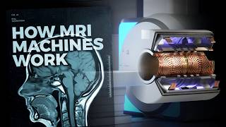
them together and hopefully having a good clear understand scanning of how MRI physics works now as you'll see here is a 3D model of the MRI machine itself and you can see it's made of multiple different layers and each one of these layers represents a different type of magnet that we're going to use to generate our image now if we look at the machine from side on and then open up that machine we can see where the patient lies within the MRI machine now MRI is different from X-ray and CT Imaging as well as ultrasound

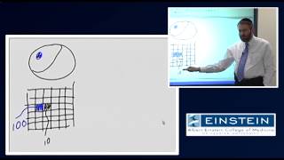
imaging in the fact that the signal that we use to generate our image is actually coming from within the patient and because the signal is coming from within the patient we need a way of localizing where exactly that signal is coming from and what we use is what's known as the Cartesian plane we can separate this image into three separate axes the first by convention is the longitudinal axis the axis that runs from head to toe along the patient and that's always labeled the Z or z-axis we can then cut the patient in transverse section

an axial plane using the X Y axis here or the X Y plane and that's what's known as the transverse plane so we've got the longitudinal plane and the transverse plane and these are really important Concepts to take forward into the upcoming talks now in MRI imaging we use a concept known as nuclear magnetic resonance we use a large magnetic field in order to induce resonance in certain atoms within the patient and in MRI imaging we use the hydrogen atom to do this now the hydrogen atom is useful one because it's abundant within the body

there are billions of hydrogen atoms within the human body and two the hydrogen atom has what's known as non-zero Spin and atoms with non-zero spin effectively act as Tiny bar magnets within the body they have a north and a South Pole and as a result have what's known as a Magnetic Moment now the Magnetic Moment In These diagrams is represented by this Arrow here now the arrow can actually be used as a vector within the MRI machine it has both Direction and magnitude and the combination of the magnetic moments amongst all the free hydrogen atoms

within the body is what's used to generate the image now in conventional MRI imaging we only use the hydrogen atom to create our MRI imaging so we can think of our patient as being a combination of multiple different hydrogen atoms that are moving randomly within the body moving with Brownian motion and the amount of movement is determined by the temperature of that patient now because hydrogen protons have a magnetic moment they will be influenced by an external magnetic field much like a compass aligns with the magnetic field of the Earth's core we can also pass

a large magnetic field across the patient that magnetic field will cause two things to happen the first is that the hydrogen atoms will align with the magnetic field and the second is that they will precess around their own axis if you think of a spinning top on a table experiencing Gravity the spinning top processes like this around its own axis the same thing is happening to these hydrogen atoms within the patient they're along the main magnetic field of our MRI scanner and they process at a certain frequency now that frequency is determined by the type

of atom so here it's hydrogen and it's determined by the strength of the magnetic field the Precision frequency is directly proportional to the strength of that magnetic field higher the magnetic field the higher the processional frequency now don't worry this is starting to confuse you we're going to look at each one of these factors in isolation in the coming talks now as you can see the hydrogen atoms either align parallel to the magnetic field or anti-parallel to the magnetic field and in fact when we look at quantum physics later the hydrogen atom itself exists in

both of these states but for now what's important is that the absolute number of hydrogen atoms that exist in the parallel Direction exceed those of that in the anti-parallel direction and those in the parallel direction are in a slightly lower energy state to those in the anti-parallel direction now we can combine these magnetic moments to create a net Magnetic Moment within the sample that we are applying this magnetic field to and as you can see there are more magnetic moments in the parallel Direction than they are in the anti-parallel direction secondly to note although the

hydrogen atoms are presetting at the same frequency they are out of phase from one another the X and Y vectors on each individual Magnetic Moment here cancel each other out you can see there's an equal distribution within the X and Y plane and what we get here is what's known as net magnetization Vector we combine all of these magnetic moments here and we get the net magnetization Vector now the net magnetization Vector is along the longitudinal axis the z-axis on the Cartesian plane there is no X or Y value here because those processional frequencies are

out of phase with one another now we mustn't think of individual hydrogen atoms when we are looking at MRI imaging we need to think of the net magnetization vector and how that is influenced by changing magnetic fields within the MRI machine so what we can do is replace these hydrogen atoms with the net magnetization Vector here now within MRI imaging what we want to measure is this net magnetization Vector but we can't measure it along the parallel Direction along the longitudinal Direction here because our main magnetic field strength is too strong and it will interfere

with our measurement of this net magnetization Vector what we want to do is move that net magnetization Vector perpendicular to our main magnetic field that will allow us to measure that signal and that's exactly what we do in MRI imaging we have our main magnetic field that is forcing those protons into the parallel Direction what we then do is apply a second magnetic field known as the radio frequency pulse now the radio frequency pulse acts in the perpendicular plane to that main magnetic field and the radio frequency pulse alternates at a frequency that is equal

to the processional frequency of the protons if the frequency of the radio frequency pulse matches that of the process additional frequency of the hydrogen atoms within the patient two things will happen the first is that the protons will start to Fan out and become more perpendicular with the main magnetic field and the second is that the processional frequencies of those protons will start to process in Phase our net magnetization Vector now will get some transverse magnetization so magnetization in the X Y plane so as we apply this radio frequency pulse that net magnetization Vector will

start gaining some transverse magnetization and the angle at which we flip that net magnetization Vector is what's known as the flip angle in this example we flipped it 90 degrees here now the protons are all processing in Phase with one another and they now align 90 degrees to the main magnetic field now what we can do is place a small coil here and the movement of a magnet as we've seen with Faraday's law of induction the movement of a magnet can induce a current and it's the movement of this net magnetization Vector that induces a

current within our receiver coil that we then use that signal to generate our image so we can see this now Vector precessing in the transverse plane in the X Y plane and we can measure a signal based on the movement of that Vector within the transverse plane now this Vector is only moving in this plane because of that radio frequency pulse and importantly that radio frequency pulse has to match the processional frequency of the hydrogen atoms if you're jumping on a trampoline and someone is jumping at exactly the same time as you you will get

double bounce you will get extra energy and you will jump higher and higher if other people are jumping on that trampoline but not at the same time they're not getting that extra energy they're bouncing the same only when those frequencies match will that energy be transferred those protons start to process in phase and the angle of magnetization will start changing and that angle changes dependent on the time of the radio frequency pulse as well as the amplitude of that radio frequency pulse now that we've moved that Vector into the transverse plane and we've generated a

signal we want to stop this radio frequency pulse now we can see the signal that has been generated here is based on that net magnetization Vector precessing at the frequency of the radio frequency pulse now we don't actually get a signal like this because what we actually do is apply a radio frequency pulse and then stop that radio frequency pulse now what actually happens is the net magnetization vectors are all processing at that radio frequency pulse and when we stop the radio frequency pulse they will start to go out of phase again and it's that

loss of phase coherence that will cause a net magnetization Vector in the transverse plane to get smaller and smaller so let's have a look at an example here here this Arrow here represents the net magnetization Vector in the transverse plane as we stop that radio frequency pulse we will see the various net magnetization vectors start to become out of phase with one another the more and more out of phase they become the less our net magnetization Vector in the transverse plane will be and we see that the signal that is generated becomes less and less

now this curve that we draw down like that is what's known as the free induction decayed curve or the t2 star curve now importantly each and every tissue within the body will have different T2 star curves or different free induction Decay curves if we look at Water the free induction Decay is very slow over time and if we look at something like bone or fat the free induction Decay is much faster and it's those differences in loss of transverse magnetization that we can use to start generating contrast within our image and we're going to look

at that more within this talk now this process is happening simultaneously with a separate independent process the loss of transverse magnetization the loss of the vector within the X Y plane is purely because of that loss of phase between the separate protons within the various different tissues and the rate at which we lose that transverse magnetization is what's known as free induction Decay now at the same time we are also gaining or regaining the longitudinal magnetization within our sample if we have the net magnetization Vector perpendicular to our main magnetic field we have lost all

of the longitudinal magnetization or the net magnetization in the z-axis as time goes by and that radio frequency pulse has been turned off what will happen is that net magnetization Vector will slowly regain longitudinal magnetization so we can see now as as time goes by we will regain some longitudinal magnetization the y-axis here is representing the amount of MZ or longitudinal magnetization along the z-axis of our Cartesian plane along the longitudinal axis of the patient now importantly as we're gaining longitudinal magnetization here we are not losing transverse magnetization because of the tilt of the protons

we lose transverse magnetization because of those protons going out of phase with one another that free induction Decay or T2 star the loss of transverse magnetization happens much quicker than this regaining of the longitudinal magnetization now as time goes by even further we get more and more longitudinal magnetization now as we can see here we are gaining longitudinal magnetization but by this point we have lost all of our transverse magnetization because although the protons have regained some longitudinal magnetization by this point they are completely out of phase with one another and all of those X

Y vectors have canceled one another out we are still now regaining longitudinal relaxation or T1 recovery along the z-axis which takes a much longer period of time now when the vectors are all aligned with the magnetic field with the main magnetic field we have regained 100 of our longitudinal relaxation now important to note that these two processes happen independently of one another if we know the free induction decay of a certain tissue we can't calculate the T1 recovery or the longitudinal recovery of that tissue they are completely independent of one another both longitudinal relaxation like

we can see here and free induction Decay happened at different rates for different tissues and it's those differing rates that we use to generate contrast within our image and lastly and what's most important to remember is we can only measure signal that is perpendicular to the main magnetic field so it's very difficult to measure longitudinal magnetization unless we flip that Vector again perpendicular to the main magnetic field now we can go about generating images by using two separate parameters that will exploit these differences in the free induction Decay or T2 star Decay and T1 recovery

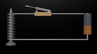
or longitudinal relaxation now the first parameter that we can use is what's known as the time of echo now I'm going to use these two knitting needles to show two separate types of tissue now we have the protons have been flipped into the longitudinal Direction in both of these tissues say CSF and fat now what happens is we apply the radio frequency pulse to 90 degrees our protons are now processing perpendicular to the main magnetic field at 90 degrees now what happens is we start to lose transverse magnetization as these start to process out of

phase with one another we lose that T2 or the free induction Decay because these are becoming out of phase within that one another they were initially in Phase providing maximum signal that signal gets lost as we get more and more out of phase now the time of echo is the time from that RF pulse at 90 degree RF pulse to the time that we actually measure the signal being generated by these tissues now given more and more time the phase incoherence will become more and more the difference between these two tissues will become more and

more so as we wait a longer period of time the difference between these two tissues will become more and more but the signal will become less and less so it's a trade-off between getting good signal and getting contrast between these two tissues now that contrast is based on the loss of transverse magnetization at the same time both of these tissues are gaining longitudinal magnetization in the z-axis and if we wait a really long period of time we can see that they will gain their longitudinal magnetization at different rates but if we wait long enough they

will gain that full net longitudinal magnetization Vector we can then flip them again to 90 degrees with a second RF pulse the time from that first RF pulse to the second RF pulse is what's known as the time of repetition or our TR time if we wait a long period of time flip it 90 degrees and then wait another period of time before measuring that signal that time to Echo time from the RF pulse to when we measure the differences in Signal are going to be based on the loss of transverse magnetization now what happens

if we wait a short period of time a short TR time we'll see that longitudinal magnetization or longitudinal relaxation occurs at different rates in fact the longitudinal or T1 recovery happens much faster than it does in water now if we wait a short period of time and don't allow the full neck longitudinal magnetization or T1 recovery to happen what we'll see is the longitudinal magnetization Vector in fat is much longer than that of water now when we apply a 90 degree RF pulse the amount of transverse magnetization will only be equal to the amount of

longitudinal recovery that has occurred so our water will have a much smaller net magnetization in the transverse plane than the fact will so when we flip this 90 degrees this is what's going to happen the signal that is being generated from fat is much more than the signal that's being generated from water the difference that we are seeing here is because of that short time of repetition it's because of the differences in longitudinal relaxation or the differences in T1 recovery so when we make our time to repetition short we're getting differences in longitudinal recovery three

or T1 differences we are not measuring the t2 differences between these two tissues now I know this is a really difficult concept and we have dedicated videos specifically looking at the types of relaxation and looking at t e and TR times what I want to give you is an idea of how we generate contrast in an image and again I'm just showing you the front cover of the puzzle that we are trying to create you don't need to understand these Concepts now but it's useful to know where we're going in future lectures now we can

manipulate the te and the TR times as I've shown you now to generate different contrast within our image as I showed you in that example with a short TR time the water lost its signal because it wasn't gaining its longitudinal relaxation as fast as the fat was and that's what's generating a T1 image where water like our CSF has a low signal and fact like the subcutaneous fattier has a high signal when we had a long time to repetition we allowed all of those tissues to fully regain their magnetization in the longitudinal plane before flipping

them into the 90 degrees and then having an echo time that measured that transverse magnetization that's what generates a T2 image where the differences between water and fat now come from the differences in the rate at which they defaze in the transverse plane water takes a very long time to de-phase and the signal remains high in the transverse plane unlike fat which because of the spin spin interactions that we're going to look at in a future talk reduces the transverse magnetization signal because fat D phases relatively quickly compared to water and we can see we

get dark signal in the fat coated axons in our white matter we get bright signal in the water in our CSF because of the differences in the t2 relaxation or the free induction Decay between those two tissues now the way in which we Act generate these images is more complicated than what we covered here but the underlying principle will always come back to the time of Echo and the time of repetition we still need to look at how we exactly go about localizing the different signals within the patient how we select certain slices along the

patient and then how we encode the different X and Y axis components of our image and in order to do this we use what is known as different pulse sequences and in this module we're going to look at the main pulse sequences the spin Echo sequence the inversion recovery sequence as well as gradient Echo sequences we will then expand on these different sequences looking at more advanced imaging techniques we'll also look at Mr spectroscopy as well as different types of angiography in MRI imaging we'll end off the module by looking at different types of MRI

artifacts as well as image quality and safety within MRI imaging now when we are generating signals Within These different pulse sequences we need a way of storing that data and then ultimately using that data to create an image now we use what is known as k space to encode for the different slices on our MRI image and we're going to spend some time looking at how we go about filling the data within a specific case space and how we can use that case space then to go about creating our image stacking those K spaces on

top of one another in order to create a scrollable image so I know this talk is very complicated and if you're new to MRI it's going to sound like a different language and that's okay each and every talk from now on is going to be looking at a specific component of what we've covered so hopefully you can use this talk as the picture on the front of the puzzle that we're trying to create and when we go about building those different sections on our puzzle the different units within this module you know where those units

fit in on the broad overarching picture now by the time I've completed this entire physics module there will be a question bank that's linked Below in the first line of the description you can use that question Bank to test yourself with actual past paper questions in Radiology physics exams I've collated all of those questions together and it's a great way for you to test your knowledge and identify knowledge gaps before heading into a radiology Physics Exam so I hope this has at least made some sense to you use this as a springboard now going into

the following modules to go and build your knowledge around MRI imaging so until the first talk where we look at the magnets in MRI imaging I'll see you there goodbye everybody