Support Vector Machines (SVM) - the basics | simply explained

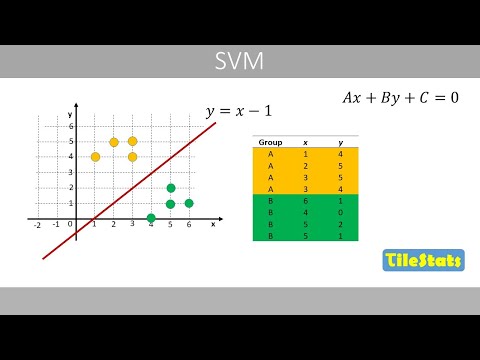
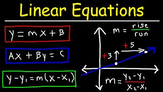
welcome to this video about support vector machines note that this video is intended for beginners with only basic knowledge in math in this video i will only assume that you are familiar with the equation of a straight line where this constant term represents that the line intercepts the y-axis at one and this number represents the slope of the line which tells us that if x increases by one unit y increases by two to really understand support vector machines you need to understand this kind of math at the end of this lecture i hope that you get the main ideas behind this math once you know this it will be a lot easier to read more advanced stuff about support vector machines we therefore see how to go from the simple equation of a straight line to this type of equation that is used in support vector machines and then see how such an equation can be used for classification usually we express the equation of a straight line like this which is called the slope intercept form because the equation contains information about the slope and the intercept of the line since this line intercepts the y axis at 1 and has a slope of 0. 5 m is here equal to 0. 5 and b is equal to 1.

for example the following horizontal line intercepts the y-axis at three and has a slope of zero since m is equal to zero the equation is y equal to three however what is the equation of the following vertical line it turns out that this form of equation cannot be used to describe a vertical line because the slope would then be infinitely large since vertical lines can be used to separate data points of two groups the slope-intercept form to describe the line is not appropriate to use in support vector machines this is one reason we need to use the so-called general form of the equation for a straight line if we move these two terms to the right hand side and divide by b we'll get the following equation well this is the slope of the line and this is the intercept we can see that the coefficient a affects the slope and the constant c affects the intercept whereas the coefficient b affects both the intercept and the slope suppose that we have the following line with a slope of 0. 5 an intercept of 1. we'll now convert this equation to the general form we therefore move all terms to the left-hand side like this to be consistent with this form we swap places of these two terms so that we have the following equation that also describes the line the coefficients are usually expressed as integers in this form if you for example multiply all terms by 4 we'll get the following equation that also describes the same line because if we solve this equation for y we'll end up with the following equation in the general form one should set the coefficient a to be a positive number which can be done by multiplying all terms with negative one so that we get the following equation that also describes the same line by using this form of the equation we can now describe this vertical line like this because x is equal to 4 along this line remember that we can describe this line with these two different forms of equations where from here on we'll focus on the second type of equation because that is the form used in support vector machines the coefficient a is equal to negative 2 and coefficient b is equal to 4 whereas c is equal to negative four let's plug in these values in this equation so we get the following equation we see that the slope is 0.

5 because if we increase one unit in x y is increased by 0. 5 and we see that the intercept is equal to 1. linear support vector machines finds the optimal values of the coefficients a and b so that the line separates the data points as good as possible we therefore first need to understand what happens with the line if we change a b and c for example if increase a from negative 2 to negative 1 the slope will be reduced from 0.

5 to 0. 25 and if you instead reduce a from negative 2 to negative 4 the slope will be increased to 1. note that when we change a the line is rotating around this point if we decrease c from negative 4 to negative eight intercept will be increased to two and if we set c to zero the intercept will be reduced to zero if instead increase b from 4 to 8 we see that the slope is reduced from 0.

5 to 0. 25 and that the intercept is reduced from 1 to 0. 5 if we now reduce b from 4 to 2 we see that the slope has increased from 0.

5 to 1 and that the intercept has increased from 1 to 2. note how the line is rotating around this point by changing the values of a and b we can move around the line like this another nice feature about this form of the equation is that it can tell us which side of the line a data point is located on if you plug in the x and y coordinates of this point in the equation we see that it results in a value that is greater than zero which in this case means that the data point is above the line in comparison this data point results in a negative value which tells us that the data point is below the line this is handy when we later will classify data points based on the equation of the line note that any data point on the line will result in a value of zero let's see what happens if we add a one to the right hand side of this equation if we then solve for y we see that the slope is the same but the intercept has increased from 1 to 1. 25 which results in the following line similarly if you add negative 1 here we'll get this line that intercepts the y-axis at 0.

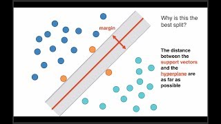
75 if we would multiply the terms on the left-hand side with these three equations with a factor smaller than one the green lines would move away from the original line which stays in the same position and if it would multiply with a factor greater than one the green lines would move closer to the original line this method is used in support vector machines to increase or decrease the so-called margin that we will discuss later on another thing we need to know before we look into the details about support vector machines is how to calculate the distance between a data point and a line the shortest distance between a data point and a line can be calculated by the following formula if you plug in the numbers from the equations of the line and the x and y coordinates of the data point and do the math we see that the distance is equal to about 2. 24 similarly the distance between two parallel lines can be calculated by the formula formula if you plug in the coefficients of the equations of the two parallel lines and the constants we see that the shortest distance between these two lines is about 2. 24 remember that we previously added a one and a negative one on the right hand side to obtain the two green lines the distance between these two green lines is calculated like this note that we have a two in the numerator because the absolute difference between the constants is always two for such lines for such lines we can simplify the equation to this or like this which you will see later on we now have a look at the real data set where we will use a support vector machine to generate a line that separates the two groups as good as possible the yellow points belong to group a which for example could represent four individuals with a certain disease whereas these green points belong to group b which could represent healthy individuals since we know which group the data points belong to we call this our training data because we let the support vector machine train on this data the training means that the support vector machine finds a line that separates the two groups in an optimal way x and y are two variables that could represent two measurements on eight individuals for example blood pressure and cholesterol level the following line is the best line to separate the two grooves based on the training data by using this line we could predict if someone has a disease or not based on the values of the two variables if the data point is below the line we predict that it belongs to group b the healthy group and if the data point is above the line we predict that it belongs to group a the disease group based on the measured values of x and y the blood pressure and cholesterol level the support vector machine can help us to predict if someone has the disease or not note that although this blue line can also separate the two groups completely it will not be good at predicting new data because if we would classify the following data point according to this blue line we will predict that it belongs to group a which means that the person is predicted to have the disease this does not make sense because the data point is much closer to the green points which represent the healthy individuals in comparison by instead using the red line we would classify the data point as belonging to group b a healthy group which seems like a better prediction because the point is closer to the green data points note that we here only have two dimensions but support vector machines work just fine also for several dimensions this means that we can use it to predict if someone has the disease or not based on many measured variables or features this is the equation of the red line which has an intercept of negative 1 and a slope of 1.

let's reformulate the equation to the form we discussed earlier we can for example multiply the terms by 4 because that does not change the position of the line remember that if you solve this equation for y we'll end up with the following equation that tells us that line has a slope of one and an intercept of negative one note that this line is called a hyperplane in support vector machines we'll now draw two parallel lines that intercept the two closest data points to the hyperplane such data points are called support vectors the equations of these two blue lines look like this for example if you plug in the x and y coordinates of a point on this blue line the left-hand side should be equal to zero which is true in this case so can we somehow normalize this equation that represents the hyperplane so that the left-hand side of this equation is equal to negative one and that the left-hand side of this equation is equal to positive one given that all three equations have the same constant term on the left-hand side as the equation of the hyperplane in other words can we find the value of k so that the left-hand side is equal to one or negative one let's plug in the x and y coordinates of this support vector like this if we solve this equation we see that we should multiply the terms on left-hand side by one over eight or simply divide the terms by eight after dividing the terms by eight the equations look like this which is the standard form of the equations in support vector machines where the right hand side is equal to positive one a negative one of the two blue lines for example if you plug in the x and y coordinates of an arbitrary point on this blue line we see that the left hand side is now equal to negative one and if you plug in the x and y coordinates of an arbitrary point on the blue line above the hyperplane we see that the left-hand side is now equal to positive one let's replace the constant 0. 5 with b note that the two distances between the red line are hyperplane and the blue lines should always be equal so that the red line is in the center this explains why we use one and negative one as constants on the right hand side the equation of the hyperplane is usually expressed like this in support vector machines this represents a vector that holds our coefficients and this is a vector that includes the variables x and y in our example t represents that we should transpose the vector w if we plug in the coefficients and x and y in this equation we see that if we multiply these two vectors we get the equation of our hyperplane note that x in this equation is a vector of the variables x and y usually one defines the two dimensions as x1 and x2 in support vector machines instead of x and y but to keep things simple i've here named the axes x and y in the standard form the equations of the three lines are defined like this which is good to know because you will see these equations a lot when you read more about support vector machines now let's use our hyperplane to classify if a data point belongs to group a yellow points or group b the green points we plug in the x and y coordinates of this data point of an arnold class in the equation of the hyperplane since this results in a negative value we predict that the data point belongs to the negative group which is group b in this case in comparison the following data point will result in a positive value which means that we predict it to belong to the positive group which is group a in this case in support vector machines one therefore divides the two groups into positive and a negative group in our example group a the yellow points is the positive group whereas group b the green points is the negative group in support vector machines y sub i usually defines the class of the training data as 1 and negative 1. for example the first data point belongs to the positive group whereas data point number five belongs to the negative group this is just another way to tell if data point in our training data belongs to group a or b the classification in support vector machines is usually defined like this we predict the class of a new observation to belong to the positive group if it is above or on the hyperplane in our example if the data point is below the hyperplane we predict that the new observation belongs to the negative group if we plug in the equation of our hyperplane and x and y-coordinates are the following data point we would see that the calculation would result in a value larger than zero which means that we will predict that the data point belongs to the positive group remember that we can calculate the distance between two parallel lines with this equation and in a special case where we have normalized equations like this we can simplify the equation to this because the absolute difference between the constant terms is always two remember that w is a vector of a and b in our example which explains why the distance between the two blue lines is usually expressed like this if there is a line that can separate the two groups completely a support vector machine tries to find the optimal values of a and b so that the distance between the two blue lines is maximized or we can also minimize the denominator because that will also maximize the distance between the two blue lines the area between the two blue lines is called the margin the support vector machine therefore tries to find a hyperplane that maximizes the width of this margin however we need some constraints because the margin can be infinitely large training the support vector machine can be defined as we try to find the optimal values of a and b of the hyperplane so that we maximize the margin so that our data points that belong to the positive group results in a value based on the equation of the hyperplane that is equal to or greater than one and that the data points that belong to the negative group results in a value that is equal to or less than negative one this means that the margin should not span beyond the data points closest to the hyperplane remember that these points are called support vectors let's see what value we get if we plug in the x and y coordinates of this data point in the equation of our hyperplane since this data point represents a support vector that is on the blue line below the hyperplane it will result in a value of negative one the width of the margin is therefore constrained so that it cannot span beyond the support vector if the hyperplane can separate the two groups completely similarly the line that defines the boundary above our hyperplane cannot be further away because if we plug in x and y coordinates of this support vector in the equation of the hyperplane that results in a value that is equal to positive one a data point that is further away will result in a value that is larger than positive one or smaller than negative one we can simplify this equation a bit if we multiply the equation by y sub i because y sub i is equal to one if the data point belongs to the positive group and equal to negative one if the data point belongs to the negative group for example this data point will now result in a positive value because we now multiply by negative 1 since this data point belongs to the negative group note that this type of problem is applicable only when the data can be fully separated by the hyperplane so what should we do if a yellow data point is down here or here we can either accept that the data point will be incorrectly classified we'll change the hyperplane so that we correctly classify all data points but with the cost of a much smaller margin remember that to maximize the margin we need to minimize what's in the denominator we can see this as we minimize only the denominator for computational reasons we usually express the term like this and to allow for misclassifications we can add this term where epsilon is a distance measure of the data points from their corresponding blue line this is called a slack variable in support vector machines in this example there is only one data point that is incorrectly classified because it is in the wrong side of the hyperplane the distance between this data point and its corresponding blue line can be described by the following equation remember that the width of the margin can be calculated by the following formula whereas half the width of the margin which is the distance between one of the blue lines and the hyperplane is calculated like this this means that epsilon will be greater than 1 for data points that are on the wrong side of the hyperplane whereas a data point within the margin but on the correct side of the hyperplane will have an epsilon value that is between 0 and 1.