T1, T2 and Proton Density Weighting | MRI Weighting and Contrast | MRI Physics Course #6

so we've looked now at T2 relaxation and T1 relaxation and how those relaxation rates occur differently within different tissues and those differing rates account for the T1 or T2 contrast differences within an image today we're going to look at how we can manipulate the pulse sequence itself in order to preferentially highlight either the T1 differences in tissues or the t2 differences in tissues and this is what's known as a weighting of an image we can create a T1 weighted image where the contrast in this image is predominantly due to the T1 relaxation differences between the

various tissues or we can create a T2 weighted image where the contrast here is because of the t2 relaxation rates that differ Within These different tissues and in the end we're going to look at a different type of weighting known as proton density weighting so to review we know that there are two separate relaxation processes happening simultaneously but independent from one another the first is transverse Decay or T2 relaxation spin spin relaxation where protons are defacing and we are losing the net transverse magnetization vector and that loss of net transverse magnetization Vector occurs at different

rates for different tissues and it's these differences in rates of loss of transverse magnetization that accounts for the t2 differences within tissues and we know that loss of 63 percent of that transfer signal is what's known as the t2 constant and the t2 constant for each tissue will be different depending on that rate of loss the second independent but simultaneous process that's occurring is what's known as T1 relaxation longitudinal recovery or spin lattice relaxation here we're getting recovery of the longitudinal magnetization vector and again that recovery happens at different rates depending on the tissue we're

looking at and the amount of time it takes to regain 67 percent of that longitudinal magnetization Vector is what's known as a T1 time constants now when we look at these graphs it can be easy to think that these processes are happening at the same period of time and this is something that many people get wrong they think that we have a longitude no magnetization Vector that's happening here in the B naught plane and we flip that longitudinal magnetization Vector 90 degrees into the transverse plane many people get confused that the rate of loss of

transverse magnetization occurs over the exact same period of time as the rate of gain of longitudinal magnetization that's not the case we lose transverse magnetization much quicker than we gain longitudinal magnetization because of those spins the phasing canceling out their X Y plane vectors and ultimately creating no Vector in the transverse plane whilst we're still recovering that longitudinal magnetization Vector you can see here the t2 time for CSF is roughly 160 milliseconds the T1 time for CSF is 2000 200 milliseconds it takes much longer to regain that longitudinal magnetization Vector so I can't actually fit

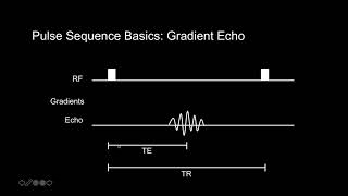
this into my slide if these were still to scale this T2 relaxation would end about here T2 relaxation happens very quickly when you compare it to T1 or longitudinal recovery now we have a basic pulse sequence here with two parameters that we can change and we've looked at these two parameters the time of Echo and the time of repetition the time of echo is the amount of time that we wait after the RF pulse to then sample that transverse magnetization signal in the coil in our MRI machine and we can change this time of Echo

and we've seen that changing the time to Echo will highlight the t2 differences within tissues then we wait a longer period of time while those tissues are gaining longitudinal recovery until we then flip again with our RF pulse the time between the first RF pulse and the next RF pulse is what's known as the time of repetition and we've seen that the time of repetition determines the amount of T1 contrast that is going to contribute to our images so let's review these two processes we've got time of echo where we're looking at the t2 relaxation

within our tissues we see initially assuming that all of these tissues have the same number of protons in them that they all start with maximum transverse magnetization signal now this is another point that we have yet to cover on fully when we apply the B naught pulse to all these tissues in our example so far we've assumed that the number of free hydrogen protons that are able to exhibit nuclear magnetic resonance in CSF is the same as what's in muscle we've assumed that this longitudinal magnetization Vector is exactly the same between these two tissues and

it's the magnitude of this longitudinal magnetization Vector that will determine the magnitude of the transverse magnetization Vector this Vector in the longitudinal plane prior to the 90 degree RF pulse will determine the vector in the transverse plane after the 90 degree RF bars now in reality there are more hydrogen free hydrogen atoms available in cs7 fat than there is in muscle and when we look at that longitudinal magnetization Vector the muscle longitudinal magnetization Vector will be less than the CSF in fat and when we flip at 90 degrees we are starting with a lower signal

now for our examples we are assuming that the number of protons available is equal and we are starting these vectors these transverse vectors at the same point here now if we were to select a short time of echo what kind of contrast would we get in the image we will get high signal but we will get very little contrast because all of those transverse magnetization vectors have yet to exhibit T2 relaxation if we wait slightly longer and measure the sample at a te with a longer te we can see now we've highlighted the differences in

transverse relaxation or transverse decay in these tissues transverse or T2 relaxation happens much slower in CSF than it does in fat and it does in muscle we can see that this signal coming from muscle is much less than that of fat and the signal coming from fat is less than that of CSF by increasing the te time we have highlighted the t2 differences in the tissue and again if we wait an even longer time to Echo we then lose contrast as well as losing signal this is useless to us because we're not getting any signal

and we're not getting any contrast and when we look at the time of repetition the time we take to allow those spins to start gaining their longitudinal magnetization before flipping them again we see that their time of repetition change will highlight the T1 differences within the tissues so we can either choose a short time of repetition or a long time of repetition so let's see what happens when we have a short time of repetition we can see that the tissues haven't regained fully their longitudinal magnetization and if we sample that tissue immediately after the 90

degree RF pulse we have a short te here the differences in these tissues is going to be predominantly because of the T1 differences if we again look at fat and we look at water and wait only a short period of time before flipping the next 90 degree rfos what exactly happens fat regains the longitudinal magnetization much faster than water does or CSF does so at this TR here fat has regained much more longitudinal magnetization in the z-axis here than water has remember at this period of time here we fully lost our transverse magnetization Vector because

these spins are out of phase with one another in CSF and in fact so our actual magnetization Vector here won't have any transverse component we will only have the longitudinal components of these magnetization vectors so for CSF it will be around here and for fact it'll be around here the degree or the magnitude of that longitudinal magnetization Vector in the longitudinal plane prior to this RF pulse here our TR is going to determine the magnitude of that transverse magnetization Vector you can see here that water if CSF is starting at a much lower transverse magnetization

than fat is and that's because it hasn't regained much longitudinal magnetization here and that highlights the T1 differences in our tissues if we wait for a longer TR you see we wait to regain all of that longitudinal magnetization Vector in the various different tissues prior to flipping 90 degrees we can see that then we lose that T1 contrast if we sample here at a short te we've got no contrast but High signal between the tissues so let's have a look at an example where we have a long TR and a short t e we've negated

the T1 differences and negated the t2 differences within null tissue this is the most basic pulse sequence that we can have a short te and a long TR with just one 90 degree RF pulse and only one time of echo what we've created here is a high signal from the longitudinal magnetization Vector we've allowed all the tissues to have a large longitudinal magnetization Vector then flip them 90 degrees and Sample straight away not allowing any of the t2 differences to occur within this tissue if we wanted to take this sequence and create a T1 weighted

image where the contrast in the image is predominantly from the T1 relaxation differences within the tissue what do we need to do to this pulse sequence we want to keep the t2 contrast out of the image so we want to keep the te time short so we don't allow any time for those T2 differences to occur the transverse relaxation to occur we don't want that to happen so we keep the te short we want to highlight the differences in T1 between the tissues so we want to reduce this TR time so look what happens I'm

going to slide this TR time along and look what happens to the contrast in the tissues as well as look what happens to this transverse magnetization Vector here we've seen that because those lower TR times don't allow for that full recovery of the longitudinal magnetization Vector they're ultimately going to affect the transverse magnetization Vector after that 90 degree RF pulse so look closely here as we reduce that TR time look at the contrast that we've now generated within our image we know that this contrast isn't due to T2 differences because we've got a very short

te it's predominantly due to the T1 differences in the tissues here the differential rates of longitudinal recovery those differing z-axis longitudinal magnetization vectors prior to the 90 degree RF flip that difference now that we're measuring at this te is because of the T1 differences in tissues and you can see now that our TR values are much lower than that 2000 value that we were looking at earlier they're in the 300 to 600 milliseconds so we've got a short TR and a very short t e in the 10 to 30 milliseconds range and this is going

to create what's known as a T1 weighted image here we can see that the CSF is dark and that's because of this longitudinal magnetization Vector having not gained very much vector magnitude here we've got a lower CSF signal intensity then we do fat intensity look how bright the subcutaneous fat is in this image and we can see we've got intermediate signal from the muscles here muscles a bit lying between the CSF and the fat and this contrast is based on the T1 differences in our image so now let's move back to that low T1 contrast

low T2 contrast but High signal if we want to bring out the t2 differences within this image we want to create a T2 weighted image we want to keep this TR along we've got high signal and very little T1 differences between the tissues at a very low TR there's very little difference in contrast between the t1s but also extremely low signal here we can't use very low TR values we need to use long TR values then if we want to highlight the t2 differences what we need to do is increase that te time and as

we increase the te time we highlight the differences in T2 relaxation transverse Decay within the various different tissues and we see that T2 relaxation happens much slower in water than it does in fat and it does in muscle and we created a different pattern of contrast here which is based on the t2 differences within our tissue we've kept the TR along at 2 000 milliseconds and we've increased the length of the te so we've got a long TR and a long te now te is now 80 to 140 milliseconds what we've created here is a

T2 weighted image where the CSF now is bright the fat has got more intermediate signal and our muscle has got low signal intensity here now you might be wondering this CSF looks like a fairly low signal why is the CSF so bright compared to the effect here now this comes back to the fact that the actual number of free hydrogen protons that are available for nuclear magnetic resonance is higher in CSF in fact than it is in other tissues like muscle or connective tissue so this y value here in the transverse magnetization plane we are

not accounting for those absolute number of proton differences so when we wait a long TR period of time here the fat and CSF will gain a large Vector our muscle Vector here will be smaller just based purely on the number of protons that are available for nuclear magnetic resonance and when we flip 90 degrees and wait for those T2 differences to occur we're going to be starting from different transverse magnetization vectors here must muscle will actually be much lower and CSF and fat will be much higher and that's why we've got brightness here but it's

clear to see here that the CSF is so much brighter in a T2 weighted image a purity two weighted image than it is in a T1 weighted image and that's because of the different t e and TR times in our pulse sequence now let's go back to this pulse sequence that we keep referring back to where we've got a long TR very little T1 differences and a short t e very little t e differences the difference is now in contrast in the tissues are going to be purely based on the number of protons that are

available for nuclear magnetic resonance we wait a long time to repetition and the differences in the longitudinal magnetization Vector here will be purely based on the number of hydrogens that are available to exhibit nuclear magnetic resonance those differences in the longitudinal magnetization Vector between the different tissues are purely based on the number of protons and when we flip it 90 degrees with the RF pulse those different is in transverse magnetization vectors are going to be purely because of the differences in the number of protons available for nuclear magnetic resonance within that specific voxel if we

sample that tissue straight away we haven't allowed those T2 differences to occur and what we've created here is contrast within our image purely based on the proton density within the image and that's what's created a proton density weighted image you can see that fat signal is bright we can see the synovial fluid here water signal is also bright that's because fats and fluid have the highest density of protons available to exhibit nuclear magnetic resonance we can see that we get great contrast within our image again if we were looking at this T2 relaxation curve we

would think that our muscle signal would be bright when we look at the muscles in this image we've got an intermediate signal here that's because as I've mentioned now multiple times this muscle signal doesn't start with such a large transverse magnetization vector it because it's longitudinal magnetization Vector was comparatively small compared to muscle and fat and when we flipped at 90 degrees it's starting at a lower y-axis value here on our T2 relaxation curves and that's why we get an intermediate muscle signal this red line should actually be lower down on our T2 relaxation curve

you can see that we get excellent contrast in this image we get very low signal from the menisci low signal from the ligaments here as well as the subchondral bone plates we can see clearly the differences between the bright fluid bright fat and those darker structures and we can see clearly the articular cartilage here now later on when we look at more advanced pulse sequences we can see how we'll be able to negate the signal from the fattier only having bright signal coming from water and that allows us to much more easily identify tears in

ligaments or in the meniscus here by seeing that contrast between the bright fluid and the surrounding low signal structures so hopefully I've convinced you now that changing the TR time will highlight the T1 differences in tissues and changing the te time will highlight the t2 differences in tissues and if we have a long TR time and a longer t e time we are going to get a T2 weighted image a shorter TR and a short te time is going to give us a T1 weighted image a combination of a long TR and a shorty will

give us what's known as a proton density weighted image now in terms of remembering the TR and t e values I haven't seen exams where you are required to remember specific values what you want is ballpark figures you'll often be given values and ask to say what type of weighting this image is now when we think of long TR times we're thinking about 2 000 milliseconds we're in the late thousands to 2000 Range when we think about t e times we are dealing with the hundreds short e times are in the tens values 10 to

30 and longer t e times are in the 80 to 160 range so if you're ever given a TR time that is within the hundreds 300 to 600 you know that that's a short TR because we're not in the late thousand to 2000 Range when you're given a te value that is closer to the hundreds range rather than the tens range we're dealing with a longer t e and as long as you can remember those kind of orders of magnitude or scale you'll be able to identify what kind of weighting you're going to be creating

in your image purely based on the TR and te values and again if you're wanting to practice these types of questions by the time I finish this entire course there will be a question Bank in the Top Line in the description that's a great place to identify the various knowledge gaps that you have and see where you need to focus your studying on now we're going to draw a line at the end of T1 and T2 differences in tissue and we're going to shift our Focus to localizing where exactly signal is coming from within the

image we'll see how we select a specific slice in our MRI and how we plot the signal values based on the X and Y plane within our image so join me in that next talk where we start to look at spatial localization in MRI images until then goodbye everybody