ESA Echoes in Space - Hazard: Flood mapping with Sentinel-1
75.91k views2523 WordsCopy TextShare
EO College
Dr. Chris Stewart explains how to derive a flood map from Sentinel-1 images, using SNAP.
SNAP: htt...
Video Transcript:
In this video we're going to use Sentinel-1 data to map flooded areas And we're going to do that by applying a very simple technique Combining an image acquired during the flood with an image applied before the flood to distinguish between flooded areas and permanent water bodies In disaster mapping applications the image acquired during the disaster event is referred to as a crisis image an image acquired before is referred to as the archive So first we will open the images by selecting the two original Sentinel-1 images in their zip format Selecting them and dragging them and
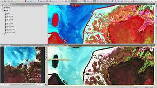
dropping them into the product Explorer window And we can see that the images were acquired in 2015 one was acquired on the 20th of March the other on the 4th of September So the 4th of September image is the crisis image and the 20th of March is the archive if we go to map of the world we can see that these images are over a part of Myanmar So let's have a look at the images if we expand the bands folder and double click on amplitude Then we can open the images in a viewer So
here we have the archive image and here the crisis So in the crisis image the flooded areas are very obvious as patches of a low backscatter return Now these dark areas are due to specular reflection over the smooth water surfaces So the signal gets reflected away from the sensor Whereas the surrounding land is much rougher and in fact we can see even an area of mountains here where we have very Rugged terrain and in fact we see a lot of distortion due to the layover and foreshortening effects So what we will do is first to
take a subset of the areas where the flooding is likely to have taken place so around the river then we will apply a multi looking in order to reduce the speckle reduce also the dimensions of the image and speed up the processing time Then we will apply a calibration which is essential to compare two images So we will go from digital numbers to a physical quantity which in this case is Sigma naught backscatter Then we will do a terrain correction to project the images onto a map system and also correct for the distortion due to
the terrain and then we will combine the images and create an RGB composite in order to distinguish between flooded areas and permanent water bodies First of all let's view the images side-by-side so we select window tile evenly And both images were applied in the same geometry so we can even see from the metadata of both images That the images were acquired while the satellite was ascending So here we can see they're both ascending and The both have the same instance angle Which is essential for flood mapping But what we notice is that there is shift
in azimut But this doesn't trouble us so much because the geometry is the same And we can cut the images to include common areas in both so here We will select the area where most flooding seems to taking place, and then we will go to Raster subset And we'll take a subset including the extent of the viewer for both images So first we have taken a subset of the crisis image now we'll take a subset of the archive by selecting the viewer here Then going to raster subset and then selecting ok These have been Saved
just to a virtual file so we do not have a real file here of the subset But what we will now do is to save these two file So we'll convert them from virtual images to real images So we go to file save product we select yes and here we can Decide an output file name, so let's remove some parts of the string of the long of the long file name that maybe we don't need and let's keep only the image acquisition date the sensor the imaging mode the polarization and the processing level I will
create a suffix here underscore crop Then we can do the same for the other image we go to a file save product we select yes to convert to BEAM-DIMAP format and Then here we take out the automatically created prefix Now we insert our own suffix removing part of the file name Calling it underscore crop Now we'll close all of the images in the product Explorer window and we will open only these two subset images And here we can see the file name that we have given these two subsets What we will now do is to
perform a multi looking in order to reduce the size of the image So we go to Radar, multi looking And in this way we also reduce the speckle So let's select a multi looking factor of three by three Clearly if we were interested in very high resolution mapping of the flooded areas we would not do a multi looking because that would reduce the resolution but In this case the floods cover quite a large area And we're interested in a low resolution map of the flooded areas so we will apply a multi looking And here we
will leave the default underscore ML as the suffix So we'll repeat this process for the other image And now we will do a calibration So we will go to radar Radiometric calibrate and this will enable us to compare the two images So here we will leave the default Sigma naught, which is the ratio instant to receive backscatter per unit area in ground range and we will select run We'll do that for both the images Now let's have a look at the images the calibrated and multi looked images So here notice how now we have Sigma
naught as the name of the band And if we double click on each then we can view them And if we select window tile evenly then we can view them side by side Notice how the images appear quite dark And if we go to the color manipulation window that we can see that many of the pixels In fact most of the pixels have a very low Backscatter value, and we have a few pixels with a very high backscatter value so it would make sense here to To convert the pixels from a linear scale to a
non linear a logarithmic scale so we call that decibel So we convert the images to decibel and then we will have a much better visualization and also a histogram that is easier to manipulate So here we right-click on the on the name of the band, and we select linear to from dB And then we select yes to create a new virtual band And we repeat that for the second image so linear to right-click linear to from dB, and we select yes Now we can view also the decibel the bands in decibel and again if we
select window tile evenly then we can compare them Simultaneously So notice how now in decibel there's a much clearer distinction between the land and the water pixels And if we look also at the histogram We can see a much easier to manipulate histogram if I can see two peaks here One peak corresponds to the pixels over land and the smaller peak corresponds to the pixels over water Finally we will do a terrain correction In order to Project the pixels onto a map system and also correct for the distortion over the areas of terrain so we
go to radar Geometric terrain correction and here we'll select Range-Doppler terrain correction Again we can leave everything is default so we will use the wgs84 geographic latitude longitude projection And then we select run we will leave the default underscore TC as the suffix Now let's have a look at the terrain corrected images But first we will convert the bands again to decibel And this time what we will do is we will convert these bands from virtual to actual bands that are written to the file so here we select convert band again by right-clicking And then
left clicking to select convert band And then we will save the image by clicking file save product and this will save the decibel band to the image We will repeat the process for the other image so here we right-click and select linear to from dB Then we right click again and select convert band and then again we save the product Now let's have a look at the terrain corrected bands in decibel So notice how the terrain has been corrected here we no longer have this distortion and we can see that the image has been projected
onto a map system we can do contrast stretch here To highlight only the pixels over the land Now we can do the same thing with the archive image And now what we're going to do is we're going to overlay one image onto the other so to do that we will create a stack and Given that the images have now been projected onto a map system We can stack these just using the product geolocation So we go to radar coregistration, stack tools, create stack And here we can select add opened and remove The images which are
not the final images Or we could also select the plus icon here and browse to the images We wish to stack which are the multi looked calibrated terrain corrected images In the create stack tab here we will select product geolocation as the initial offset method Given that we have not applied precise orbits to these images the geolocation information is good enough to overlay one images onto the other In order for them to be well registered If you want to do Interferometry then we need to do a much more precise coregistration But for this application is
enough just to overlay one image onto the other And here we will in the output tab we will remove The parts of the file name that are not common to both image, so you'll remove the acquisition date Because here, we're going to merge the images together And then we select run Now you can close this window and here we have our stacked image And now we have the The bands from each of the images put together into one image file So what we can do here is let's just open the two images in decibel and
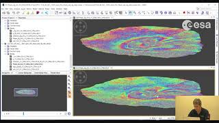
again and apply a contrast stretch What we can do is to overlay the two images in the same viewer and also create an RGB composite of the two images So here if we go to layer manager and we select the plus icon and then we go to image of band select next and here We will overlay The second image onto this one here, so here we have The 20th of March image so we will overlay the 4th of September image in decibel And then we can compare the two By selecting or deselecting this checkbox next
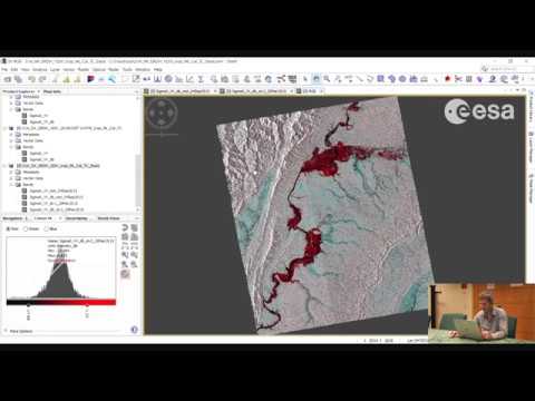
to the layer that overlays the original image Or we can select the layer here and change the transparency slider Now we're going to apply technique to distinguish between the flooded areas and the permanent water bodies And to do that we will create an RGB composite first we select the Name of the image in the product Explorer window so the name of the stack then we go to window open RGB image window We will select the archive image for the red band And we will select the crisis image for the green and the blue bands and
the reason why we do that is so that in the red channel we will have over the flooded areas a high Radar response because these areas will be land in the archive image we do not expect to see flooded areas and therefore we will have a high backscatter return However over the flooded areas will have a low backscatter return in the crisis image So where we see flooded areas? They should appear in red as will have a high response in the red channel But a low response in the green and blue channels Over surrounding areas
where we have We have no flooded areas we should see tones of gray as the backscatter should be more or less the same in red green and blue over the permanent water bodies we should have a Uniformly dark return given that will have a low backscatter return in both the archive and the crisis Therefore in red green and blue will have a low response So now we will select ok and view our flood map So here we can see quite clearly In areas of red the flooded areas And we see the river Which appears very
dark And then the surrounding areas are different tones of grey In some areas we may see some parts of the image in cyan so in the green and blue channels Where we have a higher response in the crisis image than in the archive But these may be due to a particular Ground cover, which is not related to floods Now what we can do with this flood map is To export it to a different format, so we could go to file export and select for example GeoTiff or another very quick and simple way of comparing This
flood map with with other layers is to convert it to Google Earth format And then we can overlay it onto the imagery in Google Earth So to do that we can right click inside the viewer and select export view as Google Earth kmz And here we can create a file name for this Google Earth image we can call it flood, and it will save it to kmz format And then once it is finished We can browse to the folder where we have saved the kmz file And then if we have Google Earth installed on our
computers we can just double click on this file and it will open in Google Earth Then here we can compare our flood map with the optical imagery on Google Earth either by deselecting here In the layers list or we can change also the transparency here We can also check the registration of our image so if we go to the edge for example of the image we can We can check the registration which in this case is pretty good So this is just a very simple technique for producing a flood map It's not perfect But at
least it can be carried out very simply and also very quickly and for disaster management applications time is often of the essence
Related Videos
2:13
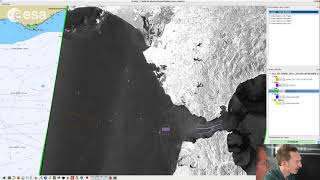
ESA Echoes in Space - Water: NRT Oil Spill...
EO College
2,222 views
26:49
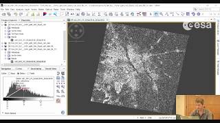
ESA Echoes in Space - Land: Urban Footprin...
EO College
25,201 views
2:09:40
NASA ARSET: Floods, Part 1/3
NASA Video
7,168 views
19:41
ESA Echoes in Space - Hazard: Volcanic eru...
EO College
21,996 views

1:20:27
Webinar 7 - Flood Mapping with Sentinel 1 ...
EO AFRICA R&D Facility
7,454 views

1:01:01
RUS Webinar: Flood Mapping with Sentinel-1...
RUS Copernicus Training
29,969 views
17:46
ESA Echoes in Space - Geometry: Introducti...
EO College
29,521 views
28:23
Flood Mapping using Sentinel-1 SAR data in...
OpenGeo Lab
28,602 views

10:56
Kamala Harris humiliated as CBS releases r...
Sky News Australia
1,778,663 views

31:28
Downloading and Preprocessing Sentinel SAR...
Pradeep Gyawali
404 views
55:24
NASA ARSET: Basics of Synthetic Aperture R...
NASA Video
165,365 views
18:09
What is under Santorini that makes it so d...
TheGeoModels
320,907 views

1:17:23
RUS Webinar: Rice Detection with Sentinel-...
RUS Copernicus Training
18,344 views

30:01
The Five 2/6/25 FULL END SHOW | ᖴO᙭ ᗷᖇEᗩKI...
İlknur çokyaman
1,546,584 views
1:08:01
RUS Webinar: Freshwater Quality Monitoring...
RUS Copernicus Training
14,500 views
24:08
ESA Echoes in Space - Water: Oil Spill map...
EO College
8,685 views
1:05:16
RUS Demo: Land Subsidence Mapping using Se...
RUS Copernicus Training
34,914 views

21:29
What if you just keep zooming in?
Veritasium
5,152,720 views

16:11
ESA Echoes in Space - Land: Crop type mapp...
EO College
45,296 views
29:20
Exploring Sentinel-2 multi-spectral band c...
GEARS - Geospatial Ecology and Remote Sensing
74,195 views