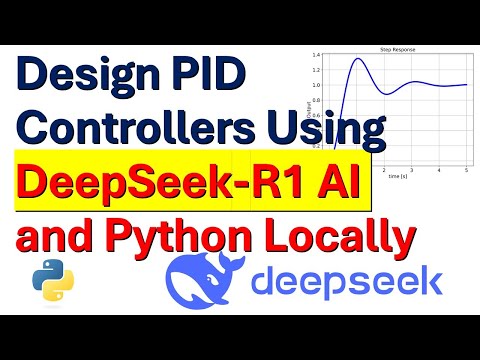
AI Revolution: Design PID Controllers Using DeepSeek-R1 AI Model and Python Locally
13.92k views2776 WordsCopy TextShare
Aleksandar Haber PhD
#deepseek #pidcontroller #robotics #mechatronics
It takes a significant amount of time and energy to...
Video Transcript:
hello everyone and welcome to machine learning Robotics and large language model tutorials in this tutorial we explain how deep seek R1 AI model and Python programming language can be used to design PID controller parameters deep seek R1 and python are running on a local computer for those of you who are not familiar with deep seek R1 here is a brief introduction deep seek R1 is maybe one of the most powerful AI reasoning models whose performance is similar to the Chad GPT models however there is one catch and big difference which motivates us to use deep seek R1 namely deep seek R1 is released under the MIT license this means that you can use deep seek R1 for commercial purposes that is you can integrate it in your application that you're developing and you can even sell that application in this tutorial we're running deep seek R1 model on a local computer in Python that is we have installed deep seek R1 locally the local installation enables you to speed up the design process it enables you better privacy then you have complete control of large language Model Behavior and you can easily integrate deep seek R1 with other software now here are the prerequisites for following this tutorial first of all you need to install deep seek R1 on your system for that purpose I created a separate video tutorial explaining how to install deep seek R1 locally in Python and windows and here is the tutorial and I will provide a link to that tutorial in the description below secondly I strongly suggest you to watch this tutorial over here that explains how to use the python Control Systems library that is you need to know how to simulate to control systems in Python in fact you don't even need to watch this particular tutorial since I will provide a detailed explanations on how to do that a link to this particular video tutorial will be provided in the description below this video so let's immediately start with explanations in this video tutorial we consider the classical control system design problem and for completeness brevity and Clarity of this video tutorial let's briefly describe it this graph shows a basic structure of the feedback control algorithm Y is the output that we measure R is the reference signal or the set point C is the controller p is the plan and D is the disturbance that affects our system the main goal of the controller is to make sure that the output of the system tracks the reference signal and over here you can see a step response of the closed loop system this is a typical step response where after some time for example after 3 seconds the system will settle and more or less the set point will will be tracked and here is a brief description of the classical control system design problem given a transfer function of the plant that is given the model of the plant P ofs design a p controller that is designed CFS such that the closed loop system has a rise time smaller than x seconds where X is a parameter defined by the user and the overshoot smaller than y sense where why is the number selected by the user that is we would like to constrain two things on this response first of all the rise time that is the time it takes for the step response to go from 10 to 90% of the steady state value should be smaller than certain number and another thing that we want to constrain is this overshoot over here the overshoot should be less than a certain amount of the value value in the steady state by doing that we make sure that the system doesn't go crazy that is that it doesn't overshoot and at the same time it has a relatively Fast Response in this video tutorial we are going to consider this test case our plant will look like this it will be a typical second order model that is it's going to have a transfer function which will look like this immediately you can see the natural and damped frequency and damping ratio from here and you can see that this system is not well damped and our problem goes like this design pad control parameters such that the closed loop system has an overshoot less than 20% and Rise time less than 1 second and we are going to use deep seek R1 to solve this problem okay let's start first of all we need need to create a python code that will call Deep seek and that will pose the question and here is the code again in order to use this code you need to install deep seek R1 on your system and again I created a video tutorial here's the video tutorial and its link will be provided in the description below so let's explain the code first of all we need to import all Lama all Lama is a framework and a pip API that's used to call large language models in our case we installed deep seek by using o Lama and consequently we are calling all Lama API to call Deep seek here we need to specify the desired model in our case we are using a distilled version of Deep seek that is we are using the model with 14b parameters and over here we specify the name of the model here to see what model models are installed on your system you need to open a command prompt and in the command prompt you need to type AMA list and over here you can see the model that I'm currently running and you need to copy and paste the name over here the next step is to ask a question and here is our question the question goes like this design a pad controller in the parallel form for the open loop plan given here that is you can just insert the plant the closed loop system should have a rise time less than 1 second and overshoot less than 20% and that's it you simply pose the question over here as a string then over here you call. chat that is you call the function that we call the model you specify the name of the model then you specify over here the structure that defines what are you trying to do your role is the user and the content is the question to ask and that's it then after that you need to extract the response namely this function will generate this data structure response to get the actual response you need to type the message then content and then over here I'm going to print the response on the screen then over here I'm going to save the response in this file the name of the the file will be output. text here vid open I'm opening this file I'm using vid open mainly because I have to ensure that after I'm I wrote everything to the file the file will be automatically closed and saved properly and this is very important and then over here once we open the file we simply write the content and that's it simple as that okay now let's run the model to run this code press and hold control shift p then search for python select interpretor click here then click on the python interpreter inside of the virtual environment and then click here and click on run python file and that's it now we are running the model now here it's always a good practice to open a task manager and to look into the computer resources over here you can see that I'm using GPU you can see the GPU usage over here and GPU memory consumption memory is almost half a little bit more than half in fact there is around 14 billion parameters currently in my GPU memory and you can see the GPU processor is working hard to compute the answer and over here you need to be patient in my case I'm running Nvidia 390 GPU and after approximately 1 minute the response is generated and here it is here I open the text file produced by the model so we can see what's written all right so I need to design pad controller in parallel form for this plant here's the plan the closed loop system should have a rise time less than 1 second and an overshoot less than 20% per.
so over here the large language model is trying to summar summarize the task and then luckily and very good the large language model was able to recognize the parallel form and to write it down and then here is the procedure you can see what's happening over here I'm not going to read everything over here the general idea here is to relate the formulas and to use them that relate the time domain specification with the polls once you compute the poles of the system then you can do pole placement or something similar to to compute the pad control parameters and you can see the complete procedure over here you can see many attempts over here there are different things being tried pole placement some matching solving different types of equations Etc note over here that we are not calling behind the scene a python tool that is we are not calling a python script that will iteratively or by using reinforcement learning try to find the correct values of the parameters everything is based on a textbook knowledge and if you go down go down go down you can see the gains over here that are being computed you can see the proportional gain you can see the integral gain and you can see the derivative gain and of course you can read everything over here if you want to learn more what are the a different attempts and how to solve this is also very good for studying control engineering okay the next step is to verify these computations by simulating the Clos Loop response now for that purpose we are going to use Control Systems library in Python Control Systems library in Python is completely free and you can install it with a single line of code and to help you to start with the python control system Library I created this tutorial and I will provide a link to that tutorial in the description below so let's go and let's write a code that will test the closed loop performance on the basis of the computed parameters so here is the python code first of all we import math plot lip then we import the control systems Library you can easily installed install Control Systems Library by typing pip install control or something similar watch my video tutorial then we are importing NPI as NP and this line over here actually is not necessary so let me erase over here I've wrote a simple function that will plot the response the input parameters are x axis Vector y- axis vectors these are the vector defining the points that need to be plotted then I have a title of My Graph I have x axis label Y axis label and I have this last string that's used to define the file name namely I will save the graph as a PhD file and over here I'm defining the figure I'm plotting the results then I'm setting the title I'm setting the X label I'm setting the Y label then I'm adjusting the thicks that is I'm adjusting the size the label size then I'm plotting the grid then I'm saving the figure note over here that I'm using 600 dots per inch and I'm showing the figure and over here is an equivalent function this function has a similar form to the first function the only difference is that this function is will be will actually plot two graph at in the same plot it's very similar first of all I'm specifying for the first and second graph x-axis coordinates Y axis coordinates for the first and second graph and the rest is the same over here I'm plotting the first and second graphs showing the plot and that's it and here comes the main part over here so here are the computer control parameters so I simply went to this script I copied proportional gain here it is then I copied integral gain here it is then I Pro copied the derivative gain then over here I'm defining S as a symbolic variable for that I'm using Control Systems library and TF function note over here that the syntax is very similar to matlb syntax then over here I'm defining an open loop transfer function here it is w and I'm printing it out and here is my controller that's parameterized by KP Ki and KD know that this is a parallel form of the pad controller and then over here I'm Computing the closed loop transfer function on the basis of this block diagram namely if you know p you know C then you know that W is p multiply by C / by 1 + p c and that's exactly that and then over here I'm simulating the response I'm simulating first of all the Clos Loop response to do that I need to call the function ct. step response I need to specify the transfer function and the time Vector then I do the same thing for the open loop system that is I'm just specifying my open loop transfer function and once I call these two functions these two time series will be generated and they they represent the step response of the closed loop system and the step response of the open loop system and then I generate three graphs first of all I'm calling the plotting function the first version to get the Clos Loop response and you can see everything over here what's being provided then I'm doing the same thing for the open loop for comparison and then finally on the same graph I'm plotting both open and Clos Loops responses and you can see it over here how it looks okay so let's save this file let's now press and hold control shift p then let's search python select The Interpreter over here let's select The Interpreter then click here and bang it's Starts Now what will happen the response will be computed and that's it okay beautiful over here you can see the step response of the Clos loop system let's verify the design specifications obviously the rise time is super small it's maybe 0.
Related Videos

22:19
What is a PID Controller? | DigiKey
DigiKey
111,951 views

15:36
Install and Run DeepSeek-R1 Locally in Pyt...
Aleksandar Haber PhD
24,511 views

14:21
Building a fully local "deep researcher" w...
LangChain
137,054 views
26:58
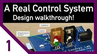
A real control system - how to start desig...
Brian Douglas
281,295 views

27:22
AI Is Making You An Illiterate Programmer
ThePrimeTime
138,802 views

10:07
Deepseek R1 Explained by a Retired Microso...
Dave's Garage
1,847,293 views

21:11
Build DeepSeek-R1 Application with GUI and...
Aleksandar Haber PhD
2,696 views
27:14
Transformers (how LLMs work) explained vis...
3Blue1Brown
4,606,555 views

14:02
Learn Ollama in 15 Minutes - Run LLM Model...
Tech With Tim
83,574 views

27:18
Explaining OpenAI's o1 Reasoning Models
Sam Witteveen
22,932 views

1:30:56
DeepSeek-R1 Crash Course
freeCodeCamp.org
261,664 views

9:49
How DeepSeek AI Helped Me Create Maps Effo...
GeoDelta Labs
812,532 views

13:37
Install and Run Locally DeepSeek-R1 AI Mod...
Aleksandar Haber PhD
64,968 views

57:45
Visualizing transformers and attention | T...
Grant Sanderson
375,570 views
30:31
US Government to BanTP-Link Devices - Live...
Matt Brown
1,466,737 views

26:52
Andrew Ng Explores The Rise Of AI Agents A...
Snowflake Inc.
514,637 views
17:54
DeepSeek-R1 Locally in Python: Install and...
Aleksandar Haber PhD
2,232 views

33:27
Diffusion Models | Paper Explanation | Mat...
Outlier
272,743 views

58:06
Stanford Webinar - Large Language Models G...
Stanford Online
106,024 views

12:10
Optimize Your AI - Quantization Explained
Matt Williams
14,314 views