The "Just One More" Paradox
3.06M views1026 WordsCopy TextShare
Marcin Anforowicz
Code I wrote for this video: https://github.com/manforowicz/Manim-Videos/blob/main/kelly_criterion.p...
Video Transcript:
Today we’ll play a game that sounds simple, but reveals a shockingly counterintuitive mathematical principle. You start with $100 and repeatedly toss a coin. Each time you flip heads, your current amount of money increases by 80%.
Each time you flip tails, it decreases by 50%. For example, you flip heads, so your $100 is multiplied by 1. 8.
Heads again, so your $180 is multiplied by 1. 8. Then tails, so your $324 is multiplied by 0.
5. And so on. You have a ½ chance of 0.
8 gain + a ½ chance of -0. 5 loss. That’s an arithmetic mean of 0.
15; a 15% average gain per coin toss. Sounds great! Would you play this game?
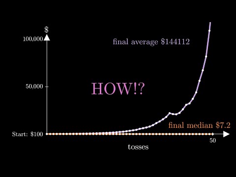
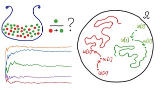
Then let’s simulate a million people, each starting with $100 and playing 50 rounds. Here’s a graph of their average wealth. As expected, their average grows exponentially.
However, their median and mode plummet to a measly $7. 2. This is called a non-ergodic system, because the population average is different from the median outcome of individuals.
But how is the median this low? Let’s visualize the problem. So, we start here, with $100.
We flip heads and multiply by 1. 8, or tails and multiply by 0. 5.
From each of these two points, we can flip heads or tails. Note that flipping 1 heads and 1 tails, already drops us down to $90. … The average increases, pulled up by the luckiest outliers.
Let’s change to a logarithmic view. Look at this point. It can be reached by any sequence of 3 heads, 3 tails.
A total of 20 sequences. Now how many sequences lead us to 4 heads and 2 tails? And so on.
Same applies to the other half. Half heads half tails occurs the most (20 times). It’s the median since it's in the center, and the mode, since it's most common.
Now let’s exit the logarithmic view. The mode slopes downward. This is shocking since every coin flip seems favorable.
Starting out, we can gain 80 or lose only 50. Here we can gain 65 or lose only 40. Here we can gain 40 or lose only 25.
This is called the “Just One More Paradox''. Each individual flip seems good, but the outcome is bad. This paradox applies to everything from gambling to social relationships to life decisions.
That’s the beauty of math. The paradox arises due to the Multiplicative nature of the game. Each flip Multiplies our entire wealth by some factor.
The lower we go, the less we can gain. What if we didn’t bet our entire wealth on each coin flip? Let’s try betting only a fixed amount of 50 dollars on each coin flip.
This is an Additive way to play the game. Note that we’re not in logarithmic view - we simply changed our strategy. Now heads always gives 40 dollars, and tails always subtracts 25 dollars, no matter where we are.
Our mode now slopes upwards, and equals the average. That’s great! But this strategy isn’t perfect.
How much should you bet if you have less than 50 dollars? What if you reach 1000 dollars? Should you raise your bet size?
Pause the video, and see if you can think of a better strategy. You might be wondering: what if we always only bet a fraction of our wealth - say ⅕, or maybe 1/10. On heads, our wealth will be multiplied by 1 plus .
8, times 1/10. On tails, our wealth is multiplied by 1 minus . 5 times 1/10.
If we flip 2 heads, and 2 tails, our expression would look like this. Or simply… If we flip 1 head, and 1 tail, it would look like this. Remember, our mode and median is flipping half heads and half tails.
This expression gives us the expected mode growth rate per coin flip! The mode will be multiplied by 1. 013 per coin flip, which is a net gain.
By the way, this is called a geometric mean. But is betting 1/10 of our wealth optimal? Why not 1/15 or ⅕?
To answer this question, we can start by generalizing our equation. Let’s say F is the fraction of wealth we’re betting, B is the gain, A is the loss, and P&Q are the probabilities of heads and tails. Now let's substitute those variables in.
And let’s graph it! The x-axis represents the fraction of wealth bet. The y-axis represents the mode growth rate.
When f=0, we’re not betting anything, so there’s no change in wealth, and our growth rate is 1. When f=1, we’re betting our entire wealth, and making a loss, so our growth rate is . 949.
However, in this highlighted segment, we’re gaining money. Highest growth rate occurs where this curve’s slope is flat. We can use calculus to find where this is.
If you don’t yet know calculus, it’s fine if you zone out for the next 20 seconds. We logarithmically differentiate with respect to r and set dr/df to zero, then solve for f. Ok, zone back in.
This equation tells us at what value of F the curve’s peak occurs. Plugging in our values gives 0. 375.
That’s the fraction of our wealth we should bet to maximize growth rate. At this fraction, the mode growth rate is 1. 028 per coin flip.
Let’s run our simulation again, having a million people each bet only . 375 of their wealth. Here’s the average… And yay!
This time the median increases steadily! All thanks to this equation, called the Kelly Criterion. Described in 1956 by John Larry Kelly Jr.
, it’s widely used by investors, specifying what fraction of wealth to bet to maximize growth rate. Give yourself a pat on the back! You’ve successfully got to the end of the video, have a better understanding of probability, and learned a new paradox!
I only had to write 1100 lines of code to animate this video, thanks to the superb Manim graphics library created by 3Blue1Brown and the community. I’d also like to thank Jason Collins for his informative blog post on ergodicity economics. Also check out the channel Mutual Information for another great explanation of the Kelly criterion.
And thanks for watching!
Related Videos
![The moment we stopped understanding AI [AlexNet]](https://img.youtube.com/vi/UZDiGooFs54/mqdefault.jpg)
17:38
The moment we stopped understanding AI [Al...
Welch Labs
925,689 views

28:24
The Two Envelope Problem - a Mystifying Pr...
Formant
591,764 views

18:55
This is How Easy It Is to Lie With Statistics
Zach Star
6,218,952 views
16:45
The Clever Way to Count Tanks - Numberphile
Numberphile
968,794 views
28:28
Russell's Paradox - a simple explanation o...
Jeffrey Kaplan
7,181,564 views

13:46
The Most Interesting Investor Who Ever Lived
Hamish Hodder
242,800 views

22:38
How To Catch A Cheater With Math
Primer
4,970,461 views
![The most beautiful equation in math, explained visually [Euler’s Formula]](https://img.youtube.com/vi/f8CXG7dS-D0/mqdefault.jpg)
26:57
The most beautiful equation in math, expla...
Welch Labs
386,684 views

33:00
The Sudoku With Only 2 Given Digits
Cracking The Cryptic
3,629,320 views

19:44
P vs. NP: The Biggest Puzzle in Computer S...
Quanta Magazine
789,613 views

30:38
Solving Wordle using information theory
3Blue1Brown
10,473,492 views

34:26
Mathematics of Maximizing Profit in Gambli...
EpsilonDelta
210,116 views
18:39
This equation will change how you see the ...
Veritasium
16,009,354 views

7:19
Would You Take This Bet?
Veritasium
7,753,026 views

24:14
The Banach–Tarski Paradox
Vsauce
44,403,356 views
15:17
What is ergodicity? - Alex Adamou
Ergodicity TV
42,203 views
8:14
The Mathematical Danger of Democratic Voting
Spanning Tree
1,021,036 views

51:03
What Voyager Detected at the Edge of the S...
Astrum
127,250 views

21:44
The weirdest paradox in statistics (and ma...
Mathemaniac
1,058,855 views

25:08
Why Going Faster-Than-Light Leads to Time ...
Cool Worlds
6,772,944 views