Matrix multiplication as composition | Chapter 4, Essence of linear algebra
3.35M views1653 WordsCopy TextShare
3Blue1Brown
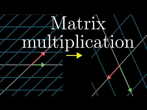
Multiplying two matrices represents applying one transformation after another.
Help fund future proj...
Video Transcript:
Hey everyone, where we last left off, I showed what linear transformations look like and how to represent them using matrices. This is worth a quick recap because it's just really important, but of course if this feels like more than just a recap, go back and watch the full video. Technically speaking, linear transformations are functions with vectors as inputs and vectors as outputs, but I showed last time how we can think about them visually as smooshing around space in such a way that grid lines stay parallel and evenly spaced, and so that the origin remains fixed.
The key takeaway was that a linear transformation is completely determined by where it takes the basis vectors of the space, which for two dimensions means i-hat and j-hat. This is because any other vector could be described as a linear combination of those basis vectors. A vector with coordinates x, y is x times i-hat plus y times j-hat.
After going through the transformation, this property that grid lines remain parallel and evenly spaced has a wonderful consequence. The place where your vector lands will be x times the transformed version of i-hat plus y times the transformed version of j-hat. This means if you keep a record of the coordinates where i-hat lands and the coordinates where j-hat lands, you can compute that a vector which starts at x, y must land on x times the new coordinates of i-hat plus y times the new coordinates of j-hat.
The convention is to record the coordinates of where i-hat and j-hat land as the columns of a matrix, and to define this sum of the scaled versions of those columns by x and y to be matrix-vector multiplication. In this way, a matrix represents a specific linear transformation, and multiplying a matrix by a vector is what it means computationally to apply that transformation to that vector. Alright, recap over, on to the new stuff.
Oftentimes, you find yourself wanting to describe the effects of applying one transformation and then another. For example, maybe you want to describe what happens when you first rotate the plane 90 degrees counterclockwise, then apply a shear. The overall effect here, from start to finish, is another linear transformation, distinct from the rotation and the shear.
This new linear transformation is commonly called the composition of the two separate transformations we applied. And like any linear transformation, it can be described with a matrix all of its own by following i-hat and j-hat. In this example, the ultimate landing spot for i-hat after both transformations is 1,1, so let's make that the first column of a matrix.
Likewise, j-hat ultimately ends up at the location negative 1,0, so we make that the second column of the matrix. This new matrix captures the overall effect of applying a rotation then a shear, but as one single action, rather than two successive ones. Here's one way to think about that new matrix.
If you were to take some vector and pump it through the rotation, then the shear, the long way to compute where it ends up is to first multiply it on the left by the rotation matrix, then take whatever you get and multiply that on the left by the shear matrix. This is, numerically speaking, what it means to apply a rotation then a shear to a given vector. But whatever you get should be the same as just applying this new composition matrix that we just found by that same vector, no matter what vector you chose, since this new matrix is supposed to capture the same overall effect as the rotation then shear action.
Based on how things are written down here, I think it's reasonable to call this new matrix the product of the original two matrices, don't you? We can think about how to compute that product more generally in just a moment, but it's way too easy to get lost in the forest of numbers. Always remember that multiplying two matrices like this has the geometric meaning of applying one transformation then another.
One thing that's kind of weird here is that this has us reading from right to left. You first apply the transformation represented by the matrix on the right, then you apply the transformation represented by the matrix on the left. This stems from function notation, since we write functions on the left of variables, so every time you compose two functions, you always have to read it right to left.
Good news for the Hebrew readers, bad news for the rest of us. Let's look at another example. Take the matrix with columns 1,1 and negative 2,0, whose transformation looks like this.
And let's call it M1. Next, take the matrix with columns 0,1 and 2,0, whose transformation looks like this. And let's call that guy M2.
The total effect of applying M1 then M2 gives us a new transformation, so let's find its matrix. But this time, let's see if we can do it without watching the animations, and instead just using the numerical entries in each matrix. First, we need to figure out where i-hat goes.
After applying M1, the new coordinates of i-hat, by definition, are given by that first column of M1, namely 1,1. To see what happens after applying M2, multiply the matrix for M2 by that vector 1,1. Working it out, the way I described last video, you'll get the vector 2,1.
This will be the first column of the composition matrix. Likewise, to follow j-hat, the second column of M1 tells us that it first lands on negative 2,0. Then, when we apply M2 to that vector, you can work out the matrix-vector product to get 0, negative 2, which becomes the second column of our composition matrix.
Let me talk through that same process again, but this time I'll show variable entries in each matrix, just to show that the same line of reasoning works for any matrices. This is more symbol-heavy and will require some more room, but it should be pretty satisfying for anyone who has previously been taught matrix multiplication the more rote way. To follow where i-hat goes, start by looking at the first column of the matrix on the right, since this is where i-hat initially lands.
Multiplying that column by the matrix on the left is how you can tell where the intermediate version of i-hat ends up after applying the second transformation. So the first column of the composition matrix will always equal the left matrix times the first column of the right matrix. Likewise, j-hat will always initially land on the second column of the right matrix.
So multiplying the left matrix by this second column will give its final location, and hence that's the second column of the composition matrix. Notice there's a lot of symbols here, and it's common to be taught this formula as something to memorize, along with a certain algorithmic process to help remember it. But I really do think that before memorizing that process, you should get in the habit of thinking about what matrix multiplication really represents, applying one transformation after another.
Trust me, this will give you a much better conceptual framework that makes the properties of matrix multiplication much easier to understand. For example, here's a question. Does it matter what order we put the two matrices in when we multiply them?
Well, let's think through a simple example, like the one from earlier. Take a shear, which fixes i-hat and smooshes j-hat over to the right, and a 90 degree rotation. If you first do the shear, then rotate, we can see that i-hat ends up at 0,1 and j-hat ends up at negative 1,1.
Both are generally pointing close together. If you first rotate, then do the shear, i-hat ends up over at 1,1, and j-hat is off in a different direction at negative 1,0, and they're pointing, you know, farther apart. The overall effect here is clearly different, so evidently, order totally does matter.
Notice, by thinking in terms of transformations, that's the kind of thing that you can do in your head by visualizing. No matrix multiplication necessary. I remember when I first took linear algebra, there was this one homework problem that asked us to prove that matrix multiplication is associative.
This means that if you have three matrices, A, B, and C, and you multiply them all together, it shouldn't matter if you first compute A times B, then multiply the result by C, or if you first multiply B times C, then multiply that result by A on the left. In other words, it doesn't matter where you put the parentheses. Now, if you try to work through this numerically, like I did back then, it's horrible, just horrible, and unenlightening for that matter.
But when you think about matrix multiplication as applying one transformation after another, this property is just trivial. Can you see why? What it's saying is that if you first apply C, then B, then A, it's the same as applying C, then B, then A.
I mean, there's nothing to prove. You're just applying the same three things one after the other, all in the same order. This might feel like cheating, but it's not.
This is an honest-to-goodness proof that matrix multiplication is associative, and even better than that, it's a good explanation for why that property should be true. I really do encourage you to play around more with this idea, imagining two different transformations, thinking about what happens when you apply one after the other, and then working out the matrix product numerically. Trust me, this is the kind of playtime that really makes the idea sink in.
In the next video, I'll start talking about extending these ideas beyond just two dimensions. See you then!
Related Videos
4:46
Three-dimensional linear transformations |...
3Blue1Brown
2,068,511 views
13:00
How AI Discovered a Faster Matrix Multipli...
Quanta Magazine
1,517,786 views

10:03
The determinant | Chapter 6, Essence of li...
3Blue1Brown
3,919,432 views
10:43
Bertrand's Paradox (with 3blue1brown) - Nu...
Numberphile
1,214,250 views

11:28
The Dot Game That Breaks Your Brain
Vsauce2
4,570,365 views

14:51
Visualize Different Matrices part1 | SEE M...
Visual Kernel
72,604 views

10:59
Linear transformations and matrices | Chap...
3Blue1Brown
5,345,932 views

51:16
Why can't you multiply vectors?
Freya Holmér
435,019 views

12:21
What's a Tensor?
Dan Fleisch
3,706,086 views

1:02:46
Grant Sanderson: 3Blue1Brown and the Beaut...
Lex Fridman
559,480 views

12:09
Inverse matrices, column space and null sp...
3Blue1Brown
2,971,308 views

35:11
Is the Future of Linear Algebra.. Random?
Mutual Information
358,548 views

19:05
Absolute Infinity - Numberphile
Numberphile
444,765 views
11:26
Do Complex Numbers Exist?
Sabine Hossenfelder
808,739 views

39:19
How Math Becomes Difficult
MAKiT
392,526 views

25:41
The deeper meaning of matrix transpose
Mathemaniac
389,018 views
17:16
Eigenvectors and eigenvalues | Chapter 14,...
3Blue1Brown
4,989,340 views

29:42
Why 4d geometry makes me sad
3Blue1Brown
912,423 views

12:37
Chaos Theory: the language of (in)stability
Gonkee
571,395 views