The F=ma of Artificial Intelligence [Backpropagation, How Models Learn Part 2]

In the early 1970s, a Harvard graduate student named Paul Worbos discovered a method for training multi-layer neural networks that we now call back propagation. Worbos would later compare the discovery to Newton's laws, positioning back propagation as a fundamental mathematical law of intelligence. When Warbos took his discovery to AI legend Marvin Minsky, Minsky rejected it outright, claiming that back propagation would not be able to learn anything difficult.

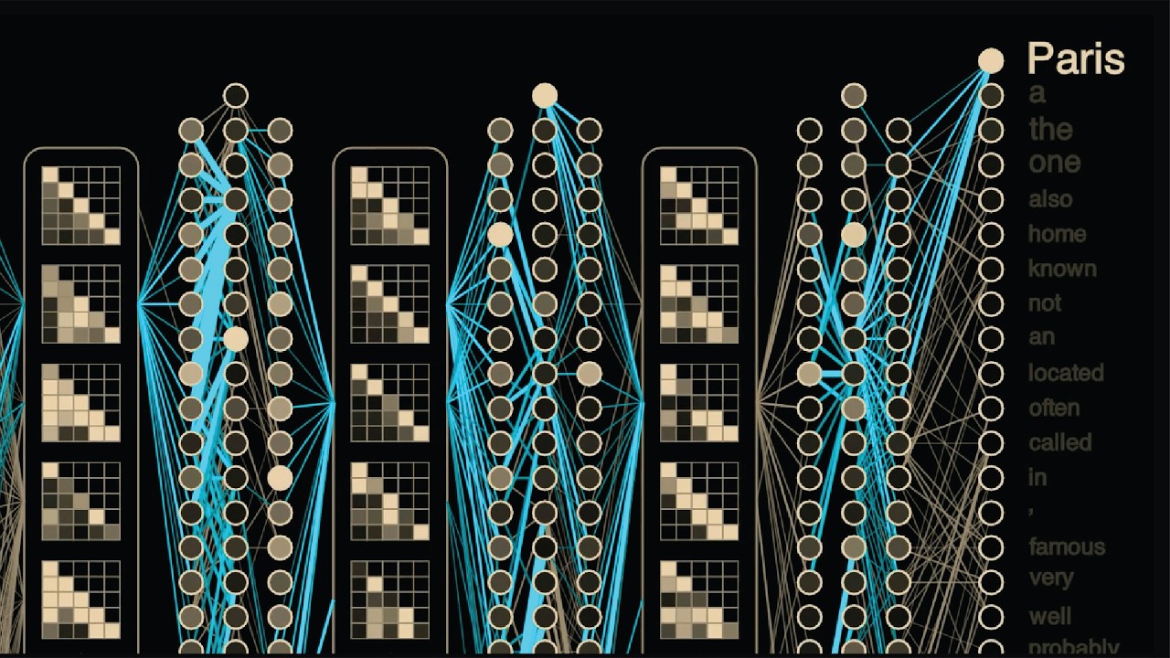
However, despite being consistently underestimated by Minsky and many others, back propagation just kept working, successfully training models to drive cars in the 1980s, recognize handwritten digits in the 1990s, and classify images with incredible accuracy in the early 2010s. And today, virtually all modern AI models are trained using back propagation. This animation shows the flow of real data through Meta's Llama 3.

2 large language model. Note that the entire model is too large to show on screen. Here we're showing the strongest connections.

Given some input text, like the capital of France is, Llama predicts the token that will come next, and the back propagation algorithm figures out how to update each of the models 1. 2 billion parameters to make Llama more confident in the correct next token. These updates are shown in blue, where thicker lines correspond to larger updates.

In this middle layer of the model, we can see back propagation is modifying the weights flowing in and out of this attention pattern. This pattern tells the model to focus on the second and fourth token in the input text. In this case, the words capital and France, which are important for predicting the next token of Paris.

Back propagation is remarkably able to figure out which parts of these massive models to update to iteratively improve performance and learn highly complex behaviors. Like Newton's laws, the back propagation algorithm is simple, elegant, and deceptively scalable, leading to incredibly rich structures and behaviors. In this video and the next in this series, we'll see precisely how back propagation works.

Now, before we get started, we need to talk about Remember when you used to be able to just ignore calls from unknown numbers? I do. It was awesome.

But now that I have kids, I've learned it's much less awesome to ignore calls from your kids school principles and doctors. But you know who never calls me anymore? Telemarketers.

Thanks to this video sponsor, Incogn, I get so few marketing calls these days that I've actually started answering unknown numbers because more often than not now, it's someone I actually need to talk to. The way Incogn does this is really impressive. After signing up for an account, you give Incogn permission to work on your behalf to contact data brokers to remove your data.

From here, you get this great dashboard that tracks all the removal requests in progress and is always working in the background. Incogn is sponsoring this whole series, which is great. And I actually had to re-record this graphic because in the few weeks since I released part one, my data has been removed from 34 more data brokers.

Incogn has just released a new feature that makes their service even more effective called custom data removals. If you Google your name and address, you may be surprised to find exactly where your personal information pops up. With custom removals, you can submit specific URLs directly to the Incogn who will work to remove your information from eligible sites.

You can get a great deal on Incogn 60% off an annual plan by using the code Welch Labs or following the link in the description below. It's been a while since I've made a multi-part series like this. Huge thank you to incogn for helping make this series possible and helping me get more quality focus time.

Now back to the back propagation algorithm. In part one of this series, we took a visual first approach to training Meta Lama 3. 2 1.

2 billion parameter model. We showed how loss landscapes give us a sense for the highdimensional spaces these models operate in, but also how these types of visualizations can fall short. In this video, we'll take a math first approach that will lead us to the back propagation algorithm that Warbos discovered over 50 years ago.

To build up the equations we need, we'll simplify our learning problem, work out the equations, and then scale back up. Instead of training a large language model like llama to predict what comes next in phrases like the capital of France is, let's train a smaller model to predict what city you're in based on your GPS coordinates. Our training data is now GPS coordinates taken from a few different cities.

Here's five coordinates from Paris and five coordinates from Madrid and Berlin. Our full Llama language model returns vectors of probabilities of length 128,256 with one entry for every token in Llama's vocabulary. Our tiny GPS model also returns vectors of probabilities but on a much smaller vocabulary of just our three cities, Paris, Madrid, and Berlin.

Instead of taking in text inputs, our tiny model will take in GPS coordinates. And we'll start by just taking in one coordinate, the longitude. So our model takes in a single numerical input, the longitude, which we'll call X.

And it returns three numbers, one probability for each city. We'll call these probabilities Yhat 1, Yhat 2, and Yhat 3. Architecturally, our model has just three total neurons, one for each city.

Each neuron's job is really simple. It multiplies its input by a learnable parameter called a weight, adds another learnable parameter called a bias, and outputs the result. Mathematically, we can write the output of our first neuron, which we'll call H1, as our first learnable parameter m1* our input x plus our bias value b1.

This model is completely equivalent to a simple linear y= mx plusb equation from high school algebra. Each of the neurons that make up artificial neural networks like llama is effectively a simple linear model like this, although with more inputs x and slopes m. And it's the job of our learning algorithm to make the appropriate adjustments to all of our m and b values to solve the larger task at hand.

Note that we're calling our output h instead of y here because we have to take one more step before reaching our final outputs yhat. Now depending on their location in the overall model, the outputs of these little linear models are sometimes passed into a few other types of functions. We know that we want the final outputs of our model Y hat to be probabilities between 0 and one.

But right now, each of our neurons are capable of returning a full range of positive and negative values. to squish the outputs of our neurons and ensure that our probabilities all add up to one. The outputs h of our final layer are typically passed into a function called softmax.

To compute the probability of Madrid yhat 1 using softmax, we raise e to the power of the output of our first neuron h1 and divide by the sum of each of the power of each of our neuron outputs h1, h2, and h3. The exponentials in the softmax equation amplify the difference between our neuron outputs, assigning more but not all probability to the neuron with the highest output value. This is why it's called a soft max.

If our Madrid, Paris, and Berlin neurons output values of 1, two, and one, our softmax operation will assign a 58% probability to yhat 2 for Paris. If our model is more confident in Paris and returns values of 1, 10, and 1, softax behaves more like our traditional maximum function, assigning Paris a probability of 99. 98%.

Softmax is the most complicated piece of math we'll encounter in this video. And happily, we'll see that when we apply some calculus and differentiate softmax, it actually gets much simpler. So, we now have all the equations we need to make predictions using our tiny GPS model.

Before training, our model weights are randomly initialized. Let's pick some simple starting values. We'll set our slope parameters to m1= 1, m2= 0, and m3= -1, and set all our bias values to zero.

If we now pass in the longitude for one of our Paris coordinates, for example, the center of the city at 2. 3514°, our positive value for M1 gives us a large H1 value of 2. 35, leading our model to incorrectly predict that we're in Madrid with a probability of 0.

91. Now, as we saw in part one, to train our model to make better predictions, we first need a way to measure our model's performance. The metric of choice for llama and many modern models is the cross entropy loss.

To compute the cross entropy loss here, we take the negative logarithm of the model's predicted probability of the correct answer. The model's current probability of pairs is only 8. 6%.

Leading to a cross entropy loss of the negative log of 0. 086 equals 2. 45.

If our model's predicted probability of Paris was 100%. Our cross entropy loss would equal the minus logarithm of 1 which equals zero. Our job from here is to change our six m and b parameters to make our loss go down.

As we saw in part one, we can do this efficiently by computing the slope of each of our parameters with respect to our loss. Combining these slopes into a vector called the gradient and using the gradient to make iterative updates to our weights. Let's now make this idea more tangible.

Let's explore as we did last time how our loss varies with a single model parameter by plotting our loss as a function of m2. Our M2 parameter in our Paris neuron currently has a value of zero resulting in a loss of 2. 45.

If we increase the parameters value to 0. 1, we can recmp compute our outputs and see that this increases our probability of being in Paris according to the model to 0. 107, reducing our loss to 2.

24. 24. Now, with these two computations of our loss for different values of M2, we've effectively estimated the value of our slope, delta L over delta M2.

This tells us that if we increase M2, our loss will go down, increasing model performance. We could theoretically do this for all six parameters in our model and use these estimated slopes to guide the gradient descent learning process. However, in practice, this numerical approach is computationally intensive.

since we have to recmp compute our outputs for each new parameter value we try and this approach can be inaccurate since we have to pick a fixed step size. Remarkably, it turns out that we can do much better the numerical estimates for these slopes. As we'll see, it's possible to exactly solve for the slopes of the loss function with respect to all parameters.

When we're done, we'll have simple equations that we can plug into directly. The fact that you can do this is not immediately obvious even to those well-versed in calculus and optimization. In the 1950s at Stanford, Bernard Widow's group trained single layer neural networks using this numerical estimate of the slope for years until Widow and his graduate student Ted Hoff stumbled onto an early version of back propagation one day in late 1959.

Even then, Widow and Hoff failed to see how to extend their method to neural networks with more than one layer. We'll see precisely how to do this after we complete our single layer example. The central idea of back propagation is to apply the rules of calculus to compute the equations for our slopes in a particularly efficient way.

Let's start with our slope delta L over delta M2. In the language of calculus, this is the partial derivative DL DM2, the rate of change of our loss L with respect to our model parameter M2. Now, we already have some equations that relate the loss to our parameter M2.

We know that our cross entropy loss is equal to the negative logarithm of our model's output probability of the correct answer yhat. This would be yhat 2 in the case of our Paris example. We can plug in our softmax equation for yhat and even go one step further and plug in the equations for each of our neurons getting a complete equation for our loss l in terms of our input x and all six model parameters.

If you're familiar with calculus, an obvious approach from here might be to compute the partial derivative we're after or dlddm2 by differentiating our expression with respect to m2. This does work, but is complex and doesn't really make use of the underlying graph structure of neural networks. Instead, it turns out that we can consider the layers of our neural network independently, solve for the rate of change through each layer, and then compose these rates of change together to much more efficiently solve for DL DM2.

Consider the simple example where we have two compute blocks. The first mapping some input x to an output y with the equation y= 2x and a second compute block mapping y to z with the equation z = 4 y. As we did with our neural network, we can put our equations together by substituting y = 2x into our second equation.

Simplifying, we see that the equation for our full system is z= 8x. The slope or derivative of this overall system equation is 8. Now, a more modular way to reach the same answer is to compute the derivative of each block individually.

Computing the slope of our first block dydx equals 2 and the slope of our second block dzy = 4. We can then multiply these rates of change together to get our overall rate of change. So, 2 * 4= 8 or dydx * dzy = dz dx.

This is known as the chain rule in calculus and scales much more cleanly to models with many layers like llama. Applying the same process to our neural network, we can break apart dlddm into dhdm* dlddh. Breaking apart the partial derivatives of our linear model and our loss and softmax function.

Now calculating the partial derivative across our logarithm and softmax function is still a bit involved. I'll put the process on screen in case you're interested and want to pause. However, the big exciting takeaway is that the result is very simple.

It turns out that the logarithm from our cross entropy loss and the exponentials from our softmax operation basically cancel out leaving us with dldh is equal to yhat minus y where yhat is a vector made up of our three output probabilities and y is a vector that equals one at the index of the correct answer and zero everywhere else. As an example, when we plug in our Paris GPS point and compute our model's probabilities, we get yhat 1 equals 0. 91 for Madrid, yhat 2= 0.

09 for Paris, and Yhat 3 rounds down to 0. 00 for Berlin. Since our ground truth label is Paris, this means that y1 equals 0, y2= 1, and y3 equals 0.

This is known as one hot encoding. So our partial derivative dlh1 from Madrid is equal to 0. 91 minus 0 equals 0.

91. This large positive value for dldh1 means that if we increase h1 our loss will increase. The partial derivative for paris dldh is equal to 0.

09 -1 = -0. 91. This large negative value means that if we increase h2 our loss will go down.

Now remember that H is just an intermediate output of our model that depends both on our model parameters and data. We've solved for DLH. But to get a derivative we can actually use to train our model like dlddm2, we need to complete our chain rule math.

Our remaining partial derivative dh2dm2 is asking us to find the rate of change of our intermediate output h2 with respect to our model parameter m2. These variables are linked by our linear equation h2= m2 * x + b2. We typically think of this equation as a line with a fixed slope of m2 and a y intercept of b2.

However, our partial derivative is asking us to think of m2 as a variable. This makes sense because learning consists of changing our parameters m and b. From this perspective, our input x is constant and m2 and h2 are variables.

This still looks like a straight line, but now its slope is equal to our input x. So the partial derivative of the output of our neuron with respect to our model parameter m2 is just the slope of our line x. Intuitively, this tells us that the impact of our model parameter m2 on our neurons output depends on the input value x.

If the input value x to our model is small, then the value of our parameter m2 matters less in our derivative calculation. and this neuron's parameters do not need to be updated as much as the model learns from this example. Alternatively, if our neuron's input X is large, it has more of an impact on our final loss and needs a larger update.

This intuition will be important as we expand to deeper models. Replacing DHDM2 with our result X, we now have a complete expression for DLDDM2. Computing DLDDM2 for our Paris example, we multiply our input longitude 2.

314° by our model's output probability of Paris 0. 9 minus one, computing a final partial derivative value of -2. 140.

So all of this back propagation mathematics is telling us that for this single pair training point, if we increase our parameter m2 by one, we expect our loss to decrease by 2. 140. Partial derivative values like this are the key result of back propagation and are the components of the gradient vector which drives the entire learning process for virtually all modern AI models.

To compute the full gradient vector for our tiny GPS model, we have to solve for five more equations, one for each remaining parameter in our model. This mathematics ends up being very similar to the process we already followed for solving for DLDDM2. Typically, these individual equations are rolled up into equations that operate on vectors and matrices instead of individual numbers.

So, we end up with a single equation to compute the partial derivatives with respect to all three M values and another single equation for all three B values. We can now use these equations to compute the partial derivatives for all six model parameters, giving us a full gradient vector. As we saw earlier, our DLDM2 value is large and negative, meaning that if we increase M2, our loss on this training example will decrease.

This makes sense because our model's predicted probability of the correct answer of Paris is low right now. And increasing M2 will increase the model's probability of Paris, lowering our loss. DLDDM1, on the other hand, is large and positive.

This means that if we increase M1, our loss will go up. This makes sense because our model's probability of the wrong answer Madrid is currently high and increasing M1 will further increase this probability increasing our loss. Since positive slopes like this mean that increasing our parameter will increase our loss.

To train our model to reduce our loss, we want to adjust our parameters in the opposite direction of our gradient. We should reduce M1 to reduce loss and increase M2 to reduce loss. Mathematically, we can do this by taking our current model parameters, subtracting a scaled version of our gradients, and replacing our parameters with the result.

This is the gradient descent process we visualized in part one as going downhill on the model's loss landscape. And thanks to back propagation, we now have an efficient way to compute our gradient vector. The scaling factor controls the size of step we take on our loss landscape and is known as the learning rate.

We generally want it to be fairly small, something like 0. 00001. This is because our gradient only gives us the slope in a very local neighborhood.

And as we saw in part one, our loss landscapes can be highly complex with slopes that quickly shift as we update our parameters. We also saw in part one how visualizing gradient descent as going downhill in our lost landscape is a fairly incomplete picture of how our model learns. Let's see if we can use our computed gradients to observe the learning process more directly.

We'll visualize our gradients as a bar around each connecting line in our model where thicker bars correspond to larger gradients. We'll use a similar approach when we visualize the gradients flowing through our full-size models later. We'll also visualize the progress as our model learns on a map.

We'll plot our current training example as a point on the map and visualize our model's outputs as a heat map on top of the map where the probability of Madrid is shown in cyan, the probability of Paris is shown in yellow and the probability of Berlin is green and brighter colors correspond to higher probabilities. Our first training point is in Paris. As we saw earlier, the initial model parameters we chose result in a high output probability for Madrid for this input longitude.

We can also see this on our map. Paris is in the blue region on our map where our model's top prediction is Madrid. This error results in high gradients for our Paris and Madrid neurons.

Moving forward one step, these high gradients lead to a reduced value of our M1 parameter and an increase in our M2 parameter, which shifts the yellow Paris region on our map a little to the right, closer to the true location of Paris. Our next training example is from Madrid, which our model mclassifies as being in Berlin, leading to high gradient values for both Madrid and Berlin. Note that on our map, these regions need to completely switch sides.

Running gradient descent for about 40 steps is enough for our gradient updates to accomplish this. Correctly classifying Madrid and Berlin and just leaving our Paris region not actually on top of Paris. Another 40 steps or so are enough for our gradients to slowly increase our M2 and B2 values, moving our model's predicted Paris region on top of the actual city.

Note that our gradients become smaller as our model learns and makes smaller errors. We can see a little more under the hood of our model by running the same training process again, but this time while visualizing the little linear models learned by each neuron. Our initially chosen slopes of 1, 0, and minus one make our initial linear models go uphill, flat, and downhill.

As our model learns, our Madrid neuron flips to pointing downhill. Our Paris neuron wobbles a bit and ends up going slightly uphill. And our Berlin neuron flips from going downhill to uphill.

If we visualize all three neurons lines on the same axis, we can see how our model is learning to use these little linear models together. For a given input longitude, the output of each neuron is equal to the height of its line on this plot. So for the Paris example with a longitude of 2.

3376°, the Madrid neurons line has a height of 2. 34. This is equal to our H1 value for this input.

Our softmax function just amplifies whichever input is largest. So whichever line is on top at a given longitude in our plot will lead to the model's highest output probability. Running our training animation again, we see that our gradients push the Madrid line, so it has the largest values over our Madrid points.

The Paris line, so it has its largest value over our Paris points, and our Berlin line, so it has the largest value over our Berlin points. In our full map view, these lines are equivalent to three planes. And through back propagation, our model learns to position each plane above the correct city.

When we apply our softmax function to the outputs of our neurons, softmax squishes and curves our planes, but retains the same general structure, resulting in our final heat map. Now, what's really compelling about back propagation is how it's able to scale to larger problems and ultimately massive language models. Let's increase the complexity of our problem and see how our intuitions and mathematics hold up.

Let's begin by adding a fourth city to our training set, Barcelona. Barcelona has a very similar longitude to Paris. So, our model now needs to take in both longitude and latitude, which we'll call X1 and X2.

We now need to expand the little linear models in our neurons to include both inputs. Meaning, we now have two slope values M per neuron. Visually, instead of a line, each neuron now looks like a little plane, where our two slope values control the steepness of the plane in each direction.

Our back propagation math works out almost exactly the same. We just have more parameters. We now have four neurons, one for each city.

Now with three parameters each with two M values that multiply each of our two inputs and a single bias value. This makes for 12 total parameters. So we need 12 derivatives to update our weights.

Training our new twoinput model, we see that it's quickly able to fit our four planes to our data and correctly divide our map into four regions. one for each city. Putting our planes together over our map, we can see how our model has fit our planes together.

So, our Madrid plane is on top of all the other planes above Madrid. Our Barcelona plane is on top above Barcelona and so on. Of course, simple planes like this can only learn a very limited set of patterns.

To see this issue more clearly, let's consider the most complex border in the world between Belgium and the Netherlands in the municipality of Barlay Hertok. These regions of the map are part of the Netherlands and these regions are part of Belgium. Given a single plane for Belgium and a single plane for the Netherlands, there's no way to cleanly divide these complex regions.

Now, it might seem a bit random to spend our time training a model to fit esoteric European borders. But this type of problem has more in common with training large language models than you may expect. Our llama model represents individual tokens like Madrid, Paris, and Berlin as vectors of48 floatingoint numbers.

When we pass in some text like the capital of France is, there's a specific length 2048 vector in our model, specifically at the final position in the residual stream that is iteratively pushed by each layer towards the vector for Paris. This gets really interesting when we consider all the different types of text that can lead to a next token of Paris, Madrid, or Berlin. If we pass in a variety of training text examples from the wiki text data set that all lead up to next tokens of Paris, Madrid or Berlin and compute the predicted next token vectors for each training example for a layer in the middle of our model, we end up with a set of length 248 vectors each generated by examples with next tokens of Madrid, Paris, or Berlin in our training set.

One way to think of these vectors is as the coordinates of our examples in the highdimensional map of language learned by our model. We can get a sense of the geometry of this map by projecting down from 248 dimensions to two using a umap algorithm which seeks to preserve the distances between points in the highdimensional space. We see some really interesting clustering in this space.

For example, this little cluster of Paris examples are all different references to the Treaty of Paris. And this little cluster are all references to George Gershwin's an American in Paris. Just as the disconnected parts of our municipality of Barlay Herto all need to map to the same country of Belgium, the disconnected regions in our space of language all need to map to the same next token of Paris.

And it's up to our model to figure out how to partition and reshape our space to achieve this. When Marvin Minsky rejected back propagation in the early 1970s, he dismissed the idea because it converged too slowly and because according to Minsky, it couldn't learn anything too difficult. Minsky was right that learning by gradient descent can take many steps.

This mattered a lot given the compute power available at the time. However, he enormously underestimated the ability of our simple back propagation algorithm to scale to solve incredibly complex problems. Next time, we'll see what Minsky missed.

Back in 2019, I completely quit Welch Labs. I had just tried going full-time creating videos, but I wasn't able to earn enough money to make it work. I got frustrated and I quit.

I went off and worked as a machine learning engineer, which was great, but I couldn't shake the feeling that I was really supposed to be making videos. Starting in 2022, I slowly eased back on Tik Tok and was able to gradually build enough momentum to take another crack at going full-time last year. When I quit in 2019, I had some time to really think about what kept pulling me back into making videos.

And I realized that deep down it was really about education. I loved math and science as a kid, but I really disliked the way I had to learn it in school. After undergrad, I really found myself questioning if I even liked math at all.

Only through my own work and study did I fall back into love with math and science years later. And now I want to use Welsh Labs to make education better. But I've realized for me to be able to do this, I have to first build a viable business.

If I can't support myself and my family, I can't spend the time I need to make this work. Last year, through sponsorships, poster and book sales, and support on Patreon, I was able to make about half of what I made as a machine learning engineer. I'm not going to lie, so far this is a much harder way to earn a living.

My goal this year is to replace my full income. This will allow me to really reach escape velocity and continue full-time on Welch Labs. Sponsorships, posters, and book sales are going well this year, but to hit my goal, I need to grow Patreon as well.

Your monthly support on Patreon would mean a lot. As a way to say thank you, today I'm launching a new reward. Starting at the $5 per month level, I'll send you a real paper cutout used in a Welch Labs video.

It comes in a nice protective sleeve with the Welch Labs logo on the front. And on the back, it says the video it came from, the release date, and a signed by me. These are a lot of fun.

I have them going all the way back to 2017. At the $5 per month level, you'll receive a smaller cutout and a larger cutout at the $10 or higher level. Cutouts ship after your first monthly payment goes through, and you'll find a link to the Watch Labs Patreon in the description below.

Huge thank you to everyone who supported Watch Labs over the years. Thanks for watching.