Feynman's (almost) impossible sum over infinite quantum paths
43.05k views4834 WordsCopy TextShare

Physics with Elliot
Compute the Feynman path integral and discover the key to quantum mechanics! 📝 Get the notes for fr...
Video Transcript:
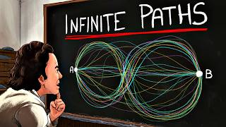
this is the Fineman path integral also known as a functional integral and if you were to ask a 100 physicists Family Feud style to name the most essential mathematical Tools in modern physics the path integral would come out at the top of the list because it's key to our understanding of everything from quantum mechanics to statistics iCal mechanics to the standard model of particle physics and in this video I'm going to show you how the path integral is defined why it's so important and how to actually compute it in an explicit example because a path
integral is not like any integral you've seen before in say your intro calculus classes with an ordinary integral like this we look at a function f of T that assigns a number to each point T along a line then the integral of the function over some range computes the area under the curve in that region and to work it out we just imagine slicing the region up into lots of skinny rectangles each one of width DT and height F of T the area of a given rectangle is then the product DT * F of T
and by summing up those contributions from all the rectangles and moreover letting their widths shrink down to be infinitesimally small we obtain the total area under the curve the integral of f but that's for an ordinary integral a path integral is a different and much more complicated Beast instead of summing over a range of points on a line we do a sum over every possible path connecting a given starting point and ending point to each path X of T we assign a number five a complex number in fact which you can think of as an
arrow in the complex plane each path gets its own Arrow where again we need to consider every possible trajectory connecting these two points by adding up those arrows for every possible path multiplied by a corresponding measure Factor DX we obtain the path integral of F and if doing a sum over an infinite set of paths sounds complicated I won't lie to you it definitely is but to begin to understand why this thing is so important for physics imagine we have a Quantum particle like an electron that starts out at this position x i at an
initial time TI then after waiting a little while at a final time TF we look for it at some other point XF Fineman showed that instead of moving along a single classical trajectory that's something like a baseball would have followed for an electron we need to consider every possible trajectory that the particle could conceivably follow and only after summing over all those trajectories in other words by Computing the path integral can we obtain the quantum mechanical probability that will find the particle at this final point when we go to measure it more precisely the probability
is proportional to the square of the path integral this schematically is fineman's path integral approach to quantum mechanics and it's kind of a wild idea when you stop to really think about it both physically and mathematically because again it says that a quantum mechanical particle doesn't follow a single path like we're used to In classical mechanics like say the parabolic Arc of a baseball flying through the air instead the particle does a kind of statistical average of every possible trajectory between the end points including paths that zigzag to the Moon in back before finally winding
up at the ending position where we observe it that's what the path integral computes and in this video I'm going to show you how to unpack what the heck it means and in doing so we'll discover the particle quantum mechanical wave function without ever even writing down the central equation of quantum mechanics the shinger equation this is actually the third in a series of videos that I've posted about the path integral and fineman's approach to Quantum Mechanics I'll begin here by taking a couple of minutes to review the main results we discovered before and then
we'll see how to put it all into practice by working through an actual path integral calculation and as usual you can get the notes that go along with this video for free at the link in the description to follow along with all the nitty-gritty details when you're ready the physics of quantum objects that is of very tiny things like electrons is very different from what we're used to to up here in our more familiar classical world like I just mentioned Quantum particles don't move along the well-defined trajectories that we see for everyday objects like baseballs
a baseball if you throw it up in the air will travel along a simple trajectory X oft where in this picture I'm graphing time on the horizontal axis and the particle position on the vertical axis it's height above the ground in this case and the result is a parabola that connects whatever initial height XI where the ball started at the initial time TI to the final height XF where we find it at any later time TF that's the classical trajectory and it's easy enough to work out by solving FAL ma with the force of gravity
pulling down on the ball importantly if we know what the ball was doing at the initial time TI we can predict precisely where we'll find it at any later time TF but quantum mechanics turns all that on its head even if we know exact L what a Quantum particle was doing at the initial time all we can predict for when we go to measure it again later on is the probability that we'll find it at some position the particle might wind up there or we might find it somewhere else and that means that in between
the particle doesn't follow a unique trajectory like the baseball did instead Fineman showed and we discovered in the previous videos that the particle averages over every possible trajectory connecting those end points and we saw how all that comes about by exploring the famous double slit experiment where we Chuck Quantum particles out a wall with two tiny holes cut into it and we see what comes out on the other side if a Quantum particle moved along a single trajectory like a baseball we could say for certain whether the particle passes through the left slit or the
right one and then we'd expect to find that most of the particles that make it through wind up somewhere in the middle like this distributed with a broad bump around the center of the back stop but that's not what happens instead we wind up with a distribution that looks something like this it's called an interference pattern with Peaks where we find lots of particles clustered together separated by valleys where Next To None arrive at all somehow each particle that travels through the barrier probes both slits at once and interferes with itself and as mind-bending as
that fact may be this simple experiment already leads to the basic idea of the path integral because if we imag imagine drilling a third hole in the barrier we'd have to include trajectories that pass through that hole as well and the same goes if we drill a fourth hole or a fifth hole and so on taking this idea to the extreme Fineman imagined filling the entire region with barriers and drilling lots of tiny holes through each of them then we'd need to consider every possible route the particle could follow bouncing from one hole to the
next on its way across the Gap and eventually we can imagine Drilling so many holes that the barriers themselves effectively disappear and we're led to the conclusion that the particle probes every possible path in getting from this initial point to whatever final point where we observe it at the detector and we need to sum over all of them that's the physical motivation behind fineman's path integral formulation of quantum mechanics to determine the probability that the particle will be found at some final position XF we need to sum over every possible trajectory that it could have
taken to get there but what exactly are we supposed to be adding up here in this sum well in the last video I explained that to each path we assign a certain complex number e to the I * s over H bar where H bar is the fundamental constant of quantum mechanics called Plank's constant and S is a number called the action that we can compute for any given path it's defined by taking the kinetic energy of the particle at any moment minus the potential energy and then integrating that difference over time along the trajectory
so we pick any path X of T connecting the initial point to the final point then we perform this ordinary integral of the kinetic energy minus the potential energy along that path and the result is a real number that we can assign to this trajectory it's action different paths will have different values for the action and therefore each term in this sum will contribute with a different weight e to the I * s over H bar which is a complex number that you can picture as an arrow in the complex plane pointing at the angle
s over har bar One path might contribute an arrow like this while another path points off in some other direction like this and according to findan we need to add up all these arrows for all the possible paths in order to predict where we'll find the particle when we go to measure it again that's all very schematic though now let's dig into the details of how we actually go about defining this sum what it can computes for us and how to evaluate it in a concrete example first of all let me State again precisely what
it is that we want to calculate here we've got this Quantum particle which is starting out at position XI at an initial time TI and the question is if we wait a little while and measure its position again later on at time TF what's the probability that will find the particle at some other point XF and here again is the answer according to findan as before we consider every possible trajectory X of T that connects these initial and final points for each path we evaluate its action s and from there we write down the corresponding
complex phase that it contributes then we do the same thing for all the other paths and we add up the complex phases that we get from each of them along with an overall factor a that will'll work out later the result is called the amplitude for the particle to propagate from point I to point f and I'll write it like this as K fi it's not quite the probability that we're looking for yet after all K here is a complex number but in general in quantum mechanics to go from an amplitude to a probability we
just need to take the absolute value and square it so that the probability we want is proportional to the absolute value of k^ squ finally what we're really looking for here is the probability that we'll find the particle within a little window around this point and so the last thing we need to do is multiply it by that tiny width dxf this is the central result of the path integral formulation of quantum mechanics and of course the hard part here is how to actually evaluate this amplitude K by summing over all the possible paths between
our initial and final points and that's what we're going to tackle now first of all the set of all these paths isn't a discrete list and so we're not actually doing a discrete sum here instead it's a path integral and so we write it like this which stands for the integral of e to the I * s/ H over the space of all paths from point I to point F but if there's an infinite Continuum of paths that go between our two points how the heck are we supposed to do a sum over all of
them well we can follow a very similar strategy to the way you learn to Define an ordinary integral in your first Calculus class with an ordinary integral we basically want to add up the values of a function F of t for each point T in a given range on a line but instead of jumping straight to summing over this Continuum of points the way we Define this thing is by breaking it up into a series of discrete steps so let's say we divide it up into n steps from TI to T1 from T1 to T2
and on and on all the way up to t n minus1 and finally our last Point TF in fact let me rename the initial Point here to t0 and the final point to TN to really make that pattern clear the total width here is TN minus t 0 and so the width of each of these smaller intervals is that total divided by n and I'll abbreviate that as delta T and now that we have a discrete list of points instead of a Continuum the problem becomes much simpler for each point we just write down the
value of the function the height in other words and we multiply it by the tiny width delta T that gives us the area of a rectangle under the curve at that point so this first one gives us an area of delta T * F of t 0 the next one has area delta T * F of T1 and so on for all the other rectangles all the way up to the last one delta T * F of t n minus1 and so we can write the total area of the rectangles as delta T * each
value of f summed over all the individual steps and that gives us a discrete approximation to the ACT actual area under the curve but now by letting the number of steps n get really big the rectangles get skinnier and skinnier until finally in the limit that n goes to Infinity we obtain the exact area under the curve this limiting expression is what we mean when we write down the definite integral of a function where the notation is meant to indicate that we're summing over the Continuum of points between TI and TF while letting the width
delta T shrink down to the infinitesimally small measure DT okay hopefully all that is mostly familiar because now we're going to apply a very similar procedure to understand the path integral so now let's return to the amplitude K where we want to integrate this quantity F over all the trajectories that connect point I to point f f here is called a functional by the way as opposed to an ordinary function it takes in a whole curve as its input and assigns a number to it compare it with an ordinary function that simply takes in one
number and returns another it's common to write functionals using square brackets like this and the whole path integral is therefore also known as a functional integral but once again instead of jumping straight to trying to sum over the Continuum of all possible paths let's start by turning it into a discrete problem so here's some trajectory X of T just like before we can take this time interval and break it up into n discreete steps from TI to T1 from T1 to T2 and so on ending with t n minus1 and the final time TF then
for each of these times the trajectory assigns a corresponding point in space X1 X2 and so on all the way up to xn minus1 and by joining those points up with straight line segments we can make a zigzag approximation to our original path and the same goes for any other path we might draw we just shift our points up or down to make a zigzag version of each new curve and in that way we can make a discrete approximation to any path that we like and so if we want to sum over all those possible
trajectories we just need to sum over all the possible values of X1 all the possible values of X2 and so on all the way up to xn minus one in other words we're going to integrate over the entire range of potential values for X1 from minus infinity all the way down to plus infinity all the way up and likewise we'll integrate over all the possible values of X2 and X3 and on and on and on until we get to xn minus one that's how we'll construct the sum over all paths by integrating over all the
possible positions of the intermediate points and like I mentioned earlier I'm also going to include an overall constant a here which we'll see will be important for actually getting a sensible answer out when we take the limit because just like before the last thing we want to do here is to take the limit as n goes to Infinity so that the time intervals between our steps become infinitesimally small and we're able to account for every possible path between the end points and this at last is how we'll Define the path integral of our functional 5
but still all this must still sound very formal so let's make it totally concrete by working out an explicit example the path integral for a free quantum mechanical particle so here again is our Quantum particle remember it started out at position XI at the initial time TI and our job is to figure out the probability of finding it at some other point XF at a later time TF according to findan the amplitude for the particle to propagate from point I to point f is given by the path integral of e to the I * the
action s / Plank's constant H bar and if we can work this integral will have answered our question because the probability is then simply determined by the modulus of k^2 so let's roll up our sleeves now and see if we can work this thing out and again to keep things as simple as possible let's assume that we're dealing with a free particle meaning that it doesn't have any forces like gravity or electromagnetism acting on it if it were a classical particle then the solution to fals ma with the force equal to zero would just be
a straight line but as we've discussed in quantum mechanics things are not quite that simple instead we need to sum over all paths weighted by e to the I * s over H bar where the action s remember is defined by taking the kinetic energy 12 mv^ 2 minus the potential energy U and integrating that difference over time along the path for a free particle though the potential energy is zero so we can throw this second term away and so what we need to do to evaluate this path integral is to write down the value
of the action s for each possible trajectory raise it to e to the I * s/ HR and finally sum over all the paths so here again is some arbitrary path like we just discussed the way we're going to handle it is by breaking it up into end discreete steps and approximating the curve as a zigzag each piece of the trajectory is then just a straight line and so it's actually not hard at all to write down the action for each segment and then add it all up to get the total take this first segment
say the total time interval here is TF minus TI and the length of each of these smaller intervals is that total divided by n and I'll call that delta T again like we did before so in this first little time interval delta T the particle starts at position XI and moves up to position X1 and since the trajectory is a straight line the speed DX by DT is constant it's just the change in the position over the change in time and constant speed means that the kinetic energy 12 mv^ 2 is constant 2 and so
when we integrate that constant over the little time interval to get the action we just get the length of time delta T times the constant value of the kinetic energy and that gives us the action for this first line segment now we just need to do the same thing for all the other line segments and then we add them all up to get the total action for the whole trajectory they all take the same form though the second one goes from X1 to X2 and so it contributes X2 - X1 2 and likewise we add
on and on from there all the way up to the last segment with XF - xn -1 2 that gives us the total action for our discretized path and raising it to e to I * s/ H bar we obtain the total weight for the path integral finally then we're ready to take this weight and plug it in to our limiting definition of the path integral which remember is given by integrating over all the intermediate values of X now I know this is a little scary looking but it's actually nowhere near as bad as it
looks because at this point we've managed to boil the whole path integral down to a handful of ordinary integrals over X1 X2 and so on and each of those ordinary integrals is something that we can evaluate exactly they're called gaussian integrals and there's a famous formula for them that you might have run into before so basically we just need to apply that formula here n-1 * over for each of these integrals over X1 X2 and so on that's not terribly exciting so for now I'll just tell you what it comes out to and I'll show
you how to get there step by step in the notes for when you're ready to tackle the details so after we do these ordinary integrals we wind up with this expression involving the positions and times and M and H bar and so on it looks a little complicated but the main thing I want you to notice right now is that the only thing that depend depends on N here is this factor which is raised to the nth power the rest has nothing to do with n at all and therefore in order for the limit where
we take the number of steps to Infinity to make sense this factor in front has got to be canceled out and that tells us that this overall constant a had better be the inverse of that factor that way all the n's disappear and at long last we're left with the exact result for the free particle p integral this is the quantum mechanical amplitude k for a free particle to propagate from position x i to XF okay but now of course we should discuss what the heck this expression actually means physically because there's an important General
lesson about quantum mechanics lurking in this formula remember that our original question here was to determine the probability of finding the particle at position XF within a little window of width dxf and to go from the amplitude to the probability we just need to take the absolute value squared times that little whip in other words the square of K tells us the probability density of finding the particle at any given point so what do we get when we take the modulus squar of our result for K well the second Factor here is of the form
e to the I * something so it has absolute value one so that doesn't contribute anything to the probability and All That Remains is this first Factor whose absolute value squared is m/ 2i H bar tfus TI this at last is the probability density for finding the particle at position XF given that it started out at position XI there's something really surprising about it though the answer doesn't actually depend on the position at all in other words if we plot this probability as a function of the final position we just get a constant horizontal line
and that means that the particle apparently has an equal chance of being being found anywhere in space but how the heck can that be the reason comes down to another fundamental principle of quantum mechanics the Heisenberg uncertainty principle which says that the more precisely we try to pin down the position of a particle in space The Wider the range of velocities it can have and since we assumed here that the particle starts off at exactly position XI its initial velocity could be absolutely anything and therefore the particle can shoot off from that initial position to
any other point in space when we go to measure it again later of course in reality we can't know the initial position of the particle exactly and so a more realistic initial setup with a window for the starting location would give us a smaller range of possible final positions and a normalizable probability distribution now there's a lot more I'd like to tell you about path integrals including the fact that the measure Capital DX isn't actually well defined but I don't want this video to become crazy long so I'll explain a bit more about some of
those details in the notes for now let me wrap up by coming back to something I mentioned at the beginning the connection between Fan's path integral approach to quantum mechanics and Schrodinger's formulation in terms of wave functions because these are not two separate theories they're just two different perspectives on the same underlying physics in fact the amplitude K that we've computed with the path integral is the wave function for a free particle that start started out at position x i to simplify a little let's suppose that the particle starts at the origin at Time Zero
then we can set XI and TI to zero and we also don't really need the final F subscripts anymore so I'll get rid of those as well then this is the wave function for this particle after we release it from the origin and in particular it had better satisfy the Schrodinger equation which says that taking the time derivative of s is the same as taking taking two derivatives with respect to X up to some constant factors so let's see if it works we just need to evaluate these two derivatives of our function s I'll let
you grab a piece of paper and compute those for yourself you should get -1 / 2T * 1 + i/ HR T x^2 all time s and a similar expression for the derivative with respect to X but with a factor of I over HR T out front then lo and behold when we simplify those factors out front we wind up with the exact same thing on either side and so this wave function does in fact satisfy the Schrodinger equation as promised but using the path integral we were able to derive it without ever even talking
about the shringer equation and just considering regular old particle trajectories albeit an infinite number of them again remember that you can get the notes for free at the link in the description that's also where you can sign up for my email newsletter to get extra b-size physics lessons delivered to your inbox thanks to all my supporters on patreon for helping to make this video possible you can join too at the link up in the corner if you'd like to see more videos like this one in the future and of course you should subscribe to the
channel hit the like button and leave a comment down below if you found this video helpful thank you so much for watching and I'll see you back here soon for another physics lesson
Related Videos

26:29
How Feynman did quantum mechanics (and you...
Physics with Elliot
553,410 views
33:37
Something Strange Happens When You Trust Q...
Veritasium
5,851,098 views

22:39
But why wavefunctions? A practical approac...
Physics with Elliot
205,075 views

20:25
A 1.58-Dimensional Object - Numberphile
Numberphile
233,990 views

4:50:40
Superconductivity and the Higgs Field
Richard Behiel
63,429 views

24:21
Ontario premier threatens to ‘shut off ele...
CNN
843,585 views

43:26
How Can Light Travel Everywhere at Once? F...
Physics Explained
252,472 views

26:08
How Google designed a smarter calculator t...
Dr. Trefor Bazett
3,166 views

37:39
Particle Physics is Founded on This Princi...
Physics with Elliot
189,638 views

17:44
Your DNA's Codes Are (Probably) From Outer...
PBS Space Time
552,845 views

19:55
SCOTUS Rules Against Trump And Saves USAID...
LegalEagle
303,414 views

31:37
Mathematicians finally find the infinite c...
Stand-up Maths
220,425 views
22:36
How Einstein Uncovered the Path a Particle...
Physics with Elliot
54,518 views

48:59
Why can't you walk through walls? The Paul...
Physics Explained
283,131 views

28:28
This Changed How I See Chemistry Forever!
FloatHeadPhysics
107,258 views

31:37
To Understand the Fourier Transform, Start...
Physics with Elliot
536,592 views

30:23
Hans Niemann Went To RUSSIA And The Reason...
GothamChess
184,862 views

28:33
Terence Tao on how we measure the cosmos |...
3Blue1Brown
2,020,962 views

21:34
The Final Barrier to (Nearly) Infinite Energy
PBS Space Time
2,540,365 views

21:45
Is English really a Germanic language?
RobWords
332,501 views