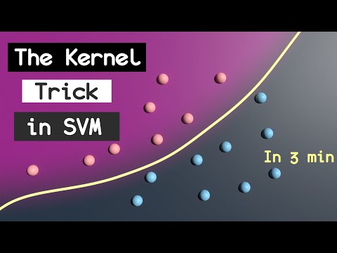
The Kernel Trick in Support Vector Machine (SVM)
266.15k views637 WordsCopy TextShare
Visually Explained
SVM can only produce linear boundaries between classes by default, which not enough for most machine...
Video Transcript:
in this video i will show you how to use kernels with this vm to perform nonlinear classification as you know svm creates a line or hyperplane to separate data points into classes the fact that the boundary between classes is flat is a pro because it makes svm easier to work with but it is also a limitation because most datasets in the real world cannot be separated by hyperplane a workaround to this limitation is to first apply a nonlinear transformation to the data points before applying svm with this technique we can easily achieve the desired effect
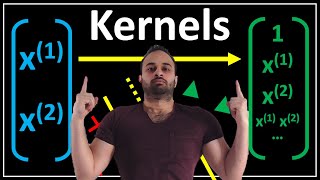
of getting a non-linear decision boundary without changing how svm works internally this is extremely easy to do in python for example we load our training data points and labels as usual but now when we call svm's fit function we don't use x but rather f x where f of x is a non-linear transformation of x geometrically this non-linear transformation might look something like this svm will return a flat hyperplane separating the two classes as usual but in the original x space this corresponds to a non-linear decision boundary mission accomplished right should we stop here and
call it today well not quite a first problem is that we need to choose what this non-linear transformation should be but as everybody knows emily enthusiasts are lazy people so the fewer choices we have to make the happier we are the second problem is that if we want a sophisticated decision boundary we need to increase the dimension of the output of this transformation and this in turn increases computational requirements the so-called kernel trick was invented to solve both of these problems in one shot the idea is that the algorithm behind this vm does not actually
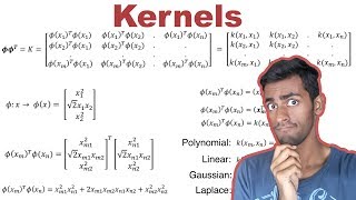
need to know what each point is mapped to under this nonlinear transformation the only thing that it needs to know is how each point compares to each other data points after we apply the nonlinear transformation mathematically this corresponds to taking the inner product between f of x and f of x prime and we call this quantity the kernel function for example the identity transformation corresponds to the linear kernel given by x transpose x prime the linear kernel gives a flat decision boundary which in this case is not good enough to separate the data properly a
polynomial transformation like this one corresponds to the polynomial kernel note that the expression of the kernel function is simple and easy to compute even though the transformation itself is complicated intuitively a polynomial kernel takes into account the original features of our data set just like that linear kernel but on top of that it also considers their interaction it takes a single line of code to use this polynomial kernel with this vm and as expected this gives a curved decision boundary sometimes it is possible to give a kernel function for which it is hard or even
impossible to find the corresponding transformation a prime example of this is the popular radial basis function kernel not only is the corresponding non-linear transformation complicated it is actually infinite dimensional so it is impossible to use directly in a computer program but the kernel expression is incredibly simple and again with a single line of code you can experiment with this kernel and you can play with this parameter gamma to make the boundary smooth or rough so in summary the kernel trick is so incredibly powerful that it feels like using a cheat code in a video game
not only it is much easier to tweak and get creative with kernels but we don't have to worry about the dimension of the output anymore thank you very much for watching and see you next time
Related Videos

20:32
Support Vector Machines Part 1 (of 3): Mai...
StatQuest with Josh Starmer
1,386,772 views

13:11
ML Was Hard Until I Learned These 5 Secrets!
Boris Meinardus
320,137 views

14:58
Support Vector Machines: All you need to k...
Intuitive Machine Learning
149,485 views

9:46
What is Kernel Trick in Support Vector Mac...
Mahesh Huddar
65,995 views
7:30
The Kernel Trick - THE MATH YOU SHOULD KNOW!
CodeEmporium
175,484 views

11:47
What the HECK is a Tensor?!?
The Science Asylum
763,019 views
12:02
SVM Kernels : Data Science Concepts
ritvikmath
73,522 views

20:18
Why Does Diffusion Work Better than Auto-R...
Algorithmic Simplicity
341,306 views

11:21
Support Vector Machines - THE MATH YOU SH...
CodeEmporium
137,219 views
8:01
Random Forest Algorithm Clearly Explained!
Normalized Nerd
615,914 views

40:08
The Most Important Algorithm in Machine Le...
Artem Kirsanov
463,258 views

15:52
Support Vector Machines Part 3: The Radial...
StatQuest with Josh Starmer
273,483 views
2:19
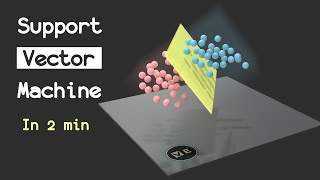
Support Vector Machine (SVM) in 2 minutes
Visually Explained
602,016 views

15:04
How I'd Learn AI (If I Had to Start Over)
Thu Vu data analytics
825,332 views
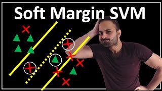
12:29
Soft Margin SVM : Data Science Concepts
ritvikmath
50,746 views
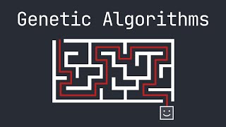
12:13
What are Genetic Algorithms?
argonaut
49,094 views
8:07
Support Vector Machines : Data Science Con...
ritvikmath
69,957 views

49:34
16. Learning: Support Vector Machines
MIT OpenCourseWare
2,009,996 views

28:44
Support Vector Machines (SVM) - the basics...
TileStats
43,700 views

4:36
106 RBF Kernel
Nanodegree India
6,953 views