Bode Plots by Hand: Real Poles or Zeros
367.76k views2387 WordsCopy TextShare
Brian Douglas
Get the map of control theory: https://www.redbubble.com/shop/ap/55089837
Download eBook on the fund...
Video Transcript:
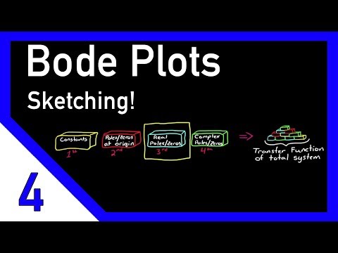
welcome back to control system lectures in this video we'll continue our discussion on sketching a Bodi plot by hand with the goal of being able to approximate the frequency response of a system that's represented by a transfer function it's important to note at this point that we're defining the building blocks of transfer functions and when these blocks are combined we can build up larger and more complex transfer functions but still be able to approximate their frequency response very easily the four different building blocks that we're discussing are constants which have no poles or zeros a
pole or zero at the origin a real Pole or zero not at the origin and a complex pair of poles or zeros all transfer functions are made up of some number of these four blocks so by learning the frequency response of each block individually it will be a simple matter of summing the responses to get the total system response in the first first video I showed you what the frequency response was for a constant and in the second video we discussed poles and zeros at the origin and now we're going to take this one step
further with real poles and zeros that aren't at the origin now there's a distinction I want to make at this point that I think's important if it doesn't make sense right now don't worry about it because I'll explain it several more times in slightly different ways in future videos but when I talk about polls and Zer I'm referring to the values of the operator s that cause the transfer function to either go to infinity or go to zero so when I say that we're looking at real poles or zeros that means that that value of
s is a real number and this number is where the pole exists in the S plane and the S plane can be graphed on a real and imaginary axis where the real component of s is Sigma and the imaginary component is Omega so we can plot s = minus1 on this graph now as you know to solve for the frequency response of a system we set the real part of s to zero and only look at the imaginary part J Omega this means we've confined ourselves to examining the system along this imaginary line only but
even though the pole or zero doesn't lie directly on the imaginary axis be sure that it is impacting the response along this line if I draw this in 3D it might make more sense as to how a pole in this case is impacting the surrounding landscape in the S plane as you can see here the J Omega line represented in pink is impacted by the pole and as we've seen before and we'll also see in this video Even though you're confining s to the imaginary line J Omega the response of the system can still have
both real and imaginary components I'll point it out when we get there let's start with a single real pole and solve for the frequency response the transfer function for a real pole can and should be written in this form 1/ 1 + S over Omega KN this form makes recognizing the break frequency Omega knot easier to do also Omega KN is sometimes referred to as the corner frequency now depending on the industry that you're in or the textbook that you're using they might not actually represent a single real pole in this form you might also
see the same exact transfer function written as Omega KN over Omega plus s or 1 over 1 + to S where too is the time constant which is 1 over Omega KN now all three of these representations are equivalent but I'm going to be referring to this blue representation for the rest of this video now I'm going to warn you at this point that the math coming up might seem intense but I assure you it's all simple algebraic steps plus it's the same steps that we did in the previous videos there's just going to be
more of them we first start with the transfer function and then set s to J Omega and at this point we're trying to separate the real component from the imaginary component and we do that by multiplying by the complex conjugate of the denominator which is just the real part minus the imaginary part and this is equal to 1 - J Omega over Omega KN over 1 + Omega 2 over Omega kn^ 2 so you can see from this solution that the real part is just one over the denominator and the imaginary part is minus Omega
over Omega KN over the denominator at this point we solve for the gain and phase of this system in the exact same way as we have done in the last video namely that gain is 20 * log base 10 of the magnitude of H of J Omega and this is just the magnitude of H of J Omega written in decb so at this point I'm just going to put the real parts and the imaginary Parts in and just sort of zip through this algebraic math I encourage you to try this on your own and go
through all of these steps one to make sure I didn't make a mistake and two I think that just practicing this helps it to sink in and that you'll remember it a little bit better but at this point we get to 1 over 1 + Omega squar over Omega not squar and the whole thing square rooted which is the magnitude of H of J Omega and when we convert this to decb this is just netive * 20 log base 10 of the square root of 1 + Omega s over Omega kn^ 2 the negative came
from the fact that this was in the denominator and we moved it to the numerator and this is just the gain equation so we can use this to plot the gain on our bod plot phase is a bit simpler it's the arc tangent of the imaginary part over the real part and when you do this math a lot of things cancel out and all you're left with is the arc tangent of negative Omega over Omega KN and this is the phase equation so with these two equations our gain equation and phase equation we can use
this to plot on our bod plot you can either plot these on a graphing program such as mat lab or you can do what we're about to do and just estimate what these graphs look like by hand and we'll do that by looking at the parts individually let's take the first case that's when Omega is much less than the break frequency Omega KN when that happens this Omega squar over Omega not squar tends towards zero so all you're left with is the square root of one and in this case the gain equation simplifies to just
-20 log base 10 of 1 which is 0 DB and we can write that on our gain plot somewhere in this area and the phase is the arc tangent of 0o which is also 0° and we can mark this point on our phase plot the second case is when Omega equals our break frequency Omega KN when that happens Omega s over Omega kn^ s equals 1 and this thing ends up being the square < TK of two so our gain is equal to- 20 log base 10 of the < TK of 2 which is equal
to-3 DB and we can estimate that point on our gain plot somewhere just below below the break frequency now for phase this is the arc tangent of Omega over Omega KN but those are equal so it's just the arc tangent of minus1 which is - 45° now the third case is when Omega is much greater than our break frequency Omega KN in this case Omega squar over Omega kn^ SAR dominates this equation it's usually much greater than one so we can rewrite this as minus 20 log base 10 of just Omega over Omega KN so
at this point every time Omega gets 10 times bigger the gain drops by minus 20 DB so we can say that this produces a line with slope of minus 20 DB per decade that intercepts the Zer DB line at Omega knot so I can just write this in here which is this green line at minus 20 DB per decade as for the the phase as Omega gets larger and larger and larger Omega over Omega KN goes towards negative infinity and I left off the negative accidentally which produces a phase ofus 90° now we have these
three points but what does the real function look like for gain I've drawn it as this yellow line which can be approximated by two line segments the first at Z DB going to Omega knot and the second starting at Omega knot and dropping off at minus 20 DB per decade for phase the real plot looks something like this which is this sloping s that starts at 0 de and goes to minus 90 estimating this is slightly trickier but can be done with three line segments first you have to find the points on the graph that
represent 1/10th of the brake frequency and 10 times the brake frequency the first Line's at 0 de and goes up to one10 of the brake frequency the next line slopes down to- 90° at 10 times the brake frequency and then it's just flat atus 90° from that point on so now when you come across a transfer function that has a single pole you can estimate the game plot with two straight lines in this manner and then you can also estimate the phase plot with just three straight lines like we've done down here now I know
I went through this pretty fast so if you have any questions on what I've done here please feel free to leave a comment in the section below and I'll try to address it so now you might have the question how can I determine the frequency response of a transfer function of a single zero without having to go through all this math again we can do it the same way that we did it on the video on poles and zeros at the origin which is that we can write a transfer function that has a real zero
as one over a real pole so the transfer function becomes one divided by 1 / 1 + S over Omega which is just a complicated way of writing 1 plus s over Omega KN and like we did before we can use the fact that we're plotting this on a log log scale bod plot to simplify this even further the real zero just becomes the negative of a real pole when you plot it on a bod plot so in that case the gain would slope up at 20 DB per decade and the phase would also gradually
increase up to positive 90° for a zero of course the best way to prove this is to actually go through the math like we did with the real zero but I'll leave that up to you if you're interested in doing that exercise let me summarize the rules for approximating the transfer function for a real Pole or zero just hopefully it syns in the first step is to write the transfer function in one of these two forms either the form for a pole or a zero depending on what you're starting with for a pole the B
plot can be approximated as follows for gain find the brake frequency Omega knot then draw a straight line at 0 DB up to Omega knot and then draw a line from there down at minus 20 DB per decade for the phase plot locate the brake frequency 10 times the brake frequency and 1/10th of the brake frequency draw a straight line at 0° to 1110th Omega knot draw a straight line at minus 90° phase starting at 10times Omega KN and going to infinity and then just connect the two lines the rules for drawing a zero are
similar they're just reflected along the horizontal axis so for the gain plot you find Omega KN you draw a straight line at Z DB to Omega KN and this time you slope up at 20 degrees per decade and for phase again you start at 0 degrees going up to 1/10th Omega but this time you jump up to positive 90° at 10 times Omega KN and then you just connect the two straight lines now at one point you might find that you have a transfer function with a single pole but you can't write it in the
form here for example this transfer function which is 1 4 plus s which has a single pole at s = -4 but you can factor out any constant gain you need in order to put the transfer function in the correct form for example 1/4 * 1 1 + S over4 where the first part of this is a constant gain and the second part is a real Pole where the breake frequency is 4 radians per second of course you can also extend this idea to a transfer function of increasing complexity by factoring out all of the
individual building blocks and writing the response for each and summing them together in the next video I'll discuss the frequency response of a transfer function with a pair of complex poles or zeros and then you'll have a complete set of building blocks with which you can build the frequency response of any transfer function I know this video got complicated at times but I appreciate you sticking through to the end and I hope that you got something from it I'll see you next time
Related Videos

11:35
Bode Plots by Hand: Complex Poles or Zeros
Brian Douglas
439,819 views

12:45
Control System Lectures - Bode Plots, Intr...
Brian Douglas
1,251,049 views

Crackling Fireplace & Smooth Jazz Instrume...
Relax Jazz Cafe
24:14
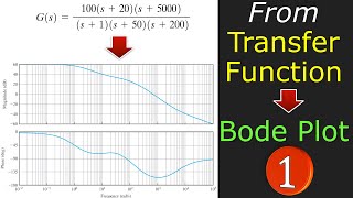
Drawing Bode Plot From Transfer Function ⭐...
CAN Education
4,936 views
12:41
Understanding Poles and Zeros in Control S...
STEM
458 views

8:51
How to Make a Real Diamond - (Not Clickbait)
JerryRigEverything
2,118,187 views
18:04
Signals and Systems - Bode Plots
UConn HKN
158,375 views

Winter Porch Ambience: Jazz, Snowfall & Cr...
Cozy Cabin Ambience

Tranquill Jazz In Lakeside | Living Coffee...
Tranquill Jazz Melody

10:56
CORRECTION: Bode Plots by Hand: Complex Po...
Brian Douglas
292,954 views

Snowfall Jazz Cafe | Slow Jazz Music in Wi...
Jazz Cafe Ambience

12:21
What's a Tensor?
Dan Fleisch
3,766,530 views

21:42
SNL WeekendUpdate 12/21/24 Saturday Night ...
Nhím Xinh Review
192,377 views
8:59
Bode Plots by Hand: Poles and Zeros at the...
Brian Douglas
619,192 views
13:53
Bode Plots Explained
Curio Res
50,724 views

Cozy Christmas Ambience 🎄 Christmas Jazz ...
Cozy Little Nook
16:42
Bode magnitude plots: sketching frequency ...
ProfKathleenWage
385,055 views

13:10
The Root Locus Method - Introduction
Brian Douglas
1,074,843 views

22:19
What is a PID Controller? | DigiKey
DigiKey
102,366 views