Use Excel to graph the efficient frontier of a three security portfolio

okay i'm gonna show you today how to graph the efficient frontier when you have more than two securities uh most of the time when you do this when people when you see people graph the efficient frontier frontier they just show one security and it's a line so what happens when it's three securities so in order to do that we have to we have let's go ahead and just get the data uh for three free three securities and uh i'm gonna use stock history i'm gonna use the excel stock history function even though it doesn't use the adjusted clothes that i preferred we just want some data anyway so i'll go for start date i'll go to i'll go equals today we'll we'll get like uh around 60 days so i'll go 61 just to get we'll go back 61 days and then we'll go equals today although today is saturday it'll go get the last day there was data usually um let's see how that works and then i'm gonna get we'll go ahead and use the tickers for tesla uh ibm i'm just picking any three i don't really care because i just want to show you how this works and then when you to use stock history i'll just go equal stock history it asks for the the stock ticker and then comma it asks for the start date comma end date and this is a spill function so it spills it spills down and it goes back 60 days and gets the close price like i told you this normally is not good to use clothes praise i like to use adjusted clothes price but but just for a demonstration we can do that on this in this video and here i'm going to go equals uh stock history i'm going to do this again because i don't want the dates so i'll go stock uh start date by the way start date we probably want to f for that because i'm going to copy this across so let me go f4 to put dollar signs and make it absolute and then the end date is here i have for that and then you put three commas and a one and that makes it so it won't show the uh date and we can copy that across since they put those dollar signs and we have the price history for for uh google tesla ibm and google so the next thing we want to do is we want to do the returns and of course we lose the data we lose a day for the returns right so i'll start down here and we'll go equals whatever google equals whatever we have here and copy that across and we'll do the daily the daily percent return is just it's pretty simple is this equal to this divided by this minus one and we see we lose this to eight two because that's why i did 61 right because i knew it's going to lose a date so so you lose it you know i can't do a2 because i don't have a day before that so it looks like it went up just a little bit so i should have a positive return right there's a little bit let's just go ahead and make that percent take it out a few places you can copy this across and send it down okay so now we have that we could call probably call this a daily return all right because because it's going by day um and then and then we're going to later on we're going to need something called the x matrix so let's go ahead and put that right here x and i'm going to go equals again just to get these carry these headers along ctrl z is your friend here something happens you don't like so x is this excess return that's going to be equal to um well you know i'm gonna get back i'll go i'll get back to x so before we before i go to x let's go ahead and do some summary statistics um so i'm just gonna go ahead and uh save time already type these out i'll just put them right here and uh so we'll also use a tesla copy this across so the expected returns is this going to be equal to the average of all all the returns for tesla right so that would be our expected returns and then we want our count because we're going to use that later so i'll go equals uh count how many observations are there and there's 43 observations we'll do the standard deviation of the returns so go equal standard deviation. sample and we get those and we'll copy that across now that's also percents let's go ahead and label it as percent and uh the variance is just equal to this squared rate probably the easiest way to do it and then we'll do what's called the modified sharp the risk the return per unit risk for each one of these securities is that divided by that right and that's a unitless number so just take it out a few places and copy that across all right so now we have some summary statistics for the for for these three and i just basically base that off of those so now we can do x that's going to be equal to the the daily return of each each test law subtract off this expected return so each one of these teslas i would subtract this expected return so i'm going to hit on this m6 i'm going to hit f4 twice because i just want the dollar sign inside the six when i copy this down i always wanted to subtract off this expected return i'm not going to have the dollar sign in front of the m because i want to move to the right when i do ibm and then then we can copy that across and send it down and so i have this all highlighted i'm going to use this later in an equation so i'm going to go so i'm going to have all this all just the numbers highlighted i'm going to go here i'm going to go capital x so i know so now whenever i go here you know i use x when i use x in an equation it's right there it goes there okay so that's that so that actually all ends up if you go here into the formula tab up here and go under name manager and added that in here okay so if i always want if i ever want to edit or remove it that's where it would go okay also and i'm going to go up here i'm going to use that in an equation so i'll call that small n and we'll call these uh standard deviation okay so whenever i use this as an equation i don't have to go highlight them it'll just go get them and that makes it very handy later all right so now we have those that information um the next thing we want to do is uh we want to do something called the variance covariance matrix and this all makes sense in a second what we're doing and so it's going to start out with a these variance covariance matrix is going to be this in this case is going to be a 3x3 so right here is going to be equal to the transpose uh these three i need a spell transplant i have a bad habit i'm not putting the s and transpose whenever you do an array function like this transpose an array function um you highlight where you want your numbers and then you have to hit ctrl shift enter you don't just hit enter you hit ctrl shift enter and it and it puts those in let's go ahead and now [Music] do that we'll go ahead and write justify that so you can see so now so now what i'm going to do i'm going to go ahead and now i'm going to put my variance covariance matrix so you can see what it is up here the variance variance current variance covariance matrix and statistic is usually the same capital sigma and it says the way i read this is x transpose x and take it times x and divided by n minus 1. so you're going to highlight where you want all your numbers to populate you need to start typing equal m multiply transpose and then we already named that x so see how when i hit x it highlights it and then we take it times x and then divide by parenthesis n minus one and then you just hit ctrl shift enter and so that's that's my variance covariance matrix and you can check if it's correct because these diagonals are the or the variances these diagonals right here and they should be the same as the variances we have right here so we know they did it correctly so we're gonna so that's the one way i always that's why i did the variance and the standard deviation because i wanted to see make sure i do it correctly and then we can do something called the correlation matrix uh just just just for informational purposes and the correlation matrix is going to be equal to we can we just form the same thing it's a three by three okay and and uh and we'll right justify that and again we're going to use this formula we see right here it's the variance covariance matrix i probably should probably let me make you type this a little bit different maybe you could call it uh now that now you know what that symbol is i tell you a sigma let me go insert sigma oop that didn't work try it again symbol double-click that wall so it's actually that this is so so before so if i want to use this in the formula let's go ahead and i'm going to highlight that and i'm going to go up here i'm going to call call it bar covar okay so i can highlight here and i'm going to do what it says here i'm going to go up barcode i'm going to go square root because i'm going to go equals square root of the var covar see how soon as soon as i finish typing it highlighted it divided by parentheses well we don't have to do parentheses we just go m multiply and the standard deviation really we already highlighted that too and called the standard deviation and we want to transpose that though right so let's go ahead and go to the front and then go transpose standard deviation and take it times the standard deviation again and then close the parenthesis on the square root then go ahead ctrl shift enter and if we did it correctly these are ones here and then so it looks like we did it correctly and um and you can see here that ibm does not uh does not correlate very well with tesla so those two would be good in a portfolio because they don't correlate very well uh tests on google and google and ibm they correlate a little bit higher um and of course they correlate exactly one to themselves okay all right so now let's go ahead and form an equally weighted portfolio and get uh and what we'll do let me move this down one i'm gonna go equals this and what we'll do um if it's equally weighted um each one of these we're gonna put a third of our money right in each one of these uh we'll go ahead and make that percent make a little bit more sense so put a third of our money in each one of these securities so to form the equally weighted portfolio is very easy it's going to be equals uh sum product it's just a it's just the uh weighted average so it's this times that plus this times that plus this times that sum product is the easiest way to do that and i'm going to go ahead and highlight that now i'm going to i'm going to use this again so i'm going to go ahead and f4 because i always wanted to subtract that expected return so it's just a as the expected return of each individual stock times how much money you put into each one that's going to be your your return your expected return on your portfolio okay and we'll go ahead and make that percent and then we can do something called the portfolio standard deviation and the portfolio standard deviation it looks like this this is the formula we use um and uh so it's just going to be equal to the weights so i'm going to go m multiply and it starts out with a weight which is these are the weights we're using and i'm going to take a times the parkour all right and then i have to multiply it again so i'm going to go ahead and multiply and go to the end i'm going to take that times the transpose of the weights again close the parentheses and then finally we have to do we have to take the square root of that so i'm gonna go to the put put everything around the parentheses around everything and go square root again you have to hit ctrl shift enter because it has array formulas in there i'm not sure what i did wrong i probably forgot a parenthesis and you get um let's go ahead and let's cop copy that and make a percent also so you get 0.

9768 percent they put the formula over here so that's what that looks like okay and then we can also do like a modified sharp ratio of the ret the just like we did up above this divided by this so for my portfolio and that's that's unitless let's go ahead and do it like that so we can see right away if we use any if we do if we decide to diversify our sharpe ratio becomes . 09 and our in our standard deviation for our portfolio is less than any of the individual basically that's why they called diversification of a free lunch because just by taking our money and spreading it out amongst three securities we decreased our risk in this case by half we but it's actually lower than any of the risk we had if we would have um you know this is the risk just for each individual security this is lower than any of those three so that's pretty cool but the nice thing is what we could say what can we do better right so let's just go ahead and take this uh i'm gonna copy it down and uh maybe excel can figure this out and get a little bit better let's try to do um let's just try to let's try excuse me cancel okay so um so i want to do the minimum variance we'll waited for the minimum variance and the way you do that is um let me get rid of this let me move this up save a little bit of space okay so solver can figure out the minimum variance portfolio um so what i'm going to do is i'm going to go to a data and solver and we want to minimize what we want to minimize we want to minimize this this standard deviation that's the same thing as minimizing the variance and we want to change these weights right here and the only constraint we want to add probably i'm going to hit i don't have to hit calls because up we want to make sure these sum up right we want to check them let me go to the home we'll do autosum and an autosum uh when we do this we have to make sure they sum up to 100 right so let's try that again so now i'm going to go to data solver and i want to set this to a minimum and then i want to add add some constraints i want to say that this this should equal one so i need to use all my money and then i'm gonna go okay and then go solve and it thinks for a second and it says okay um if you put 13 per cycle if you had a thousand dollars you put 135 dollars and 20 cents here 580 hundred eighty four dollars and sixty four cents of uh of uh tesla stock for ibm stock and two hundred and eighty thirty dollars and thirty cents of uh you know maybe i should move this down because that way we can put the little labels here so it makes so you can see what it is okay so that's how much more money we would put in each so so what did we get we got we got a return it's uh our expected return is higher than these two um tesla has a little bit higher than but but are better but our risk is way lower than the risk that we had um here right so that's one thing we could do now we could also do this let's do this uh we go copy paste and let's try doing uh let's try maximizing the sharp so i will maximize um so we can use solver so solver can do a lot of different stuff so let's try maximizing the sharpe ratio now so now i'm going to go to solver when i do when i use solver on different areas i like to reset this to make sure i don't forget anything so we want to so this is so what we i'm going to click here and i want to maximize my sharp modified sharp ratio and i have maximized by changing these weights and again we're going to add that constraint that we always have to add that constraint to add up to one just for fun let's allow short selling so i'm going to take this off and i'll go solve okay so now now it says um now it says to short google so borrow google shares and then you borrow some shares of google and then you sell them and sell those shares immediately and use it use that money to buy more shares over here and then when you close your position you sell these sell those shares go back and buy those shares of google then they went down on price now and then give the shares a google back right that's how you would short so so if you do that you know we could probably do a daily return this is per day right uh per day um per year would be equal to um one plus this to the we'll go and we'll say 252 trading days minus one so a yearly return let's make that percent so this would be the yearly okay so let's copy this formula down ctrl c ctrl v control v so now we have 100 and that's a crazy return right but you'd have to short right and i don't know if you most people aren't really interested in shorting um but but that's what would you literally return a few short your effective really return so um if you held it for a year and did that which would be now remember all this data is based off history right you don't know what's going to happen in the future this is all based off what happened in the past so we got that caveat so let's try it without shorting so let's go back to data so all i'm going to do is i'm going to click this and make sure that the weights are all positive so without shorting it says to put about 70 percent of your money in tesla and about 30 of your money in ibm so we got a really good okay so what happened up here you know it's all right so we got a really good sharp ratio that's higher than way higher than any of our individual sharp ratios right well no a little bit higher but then our portfolio of risk is is pretty good right so we're able to get our portfolio our rest down so anyway you could do some other thing you could even say uh let's go back to solver let's keep where we don't like that level of risk so i can add another constraint i could say let's also keep our portfolio of rest let's keep it less than um what's the lowest risk we have up here less than less less than or equal to whatever is on ibm so you go okay and go solve and uh so this is what it tells you to do in that case so we have the risk the set is what ibm's risk is and and this is the weights you'd use so i think you get the idea solver is very powerful and it actually really quickly finds i'm doing you know it finds uh it optimizes your portfolio but but we still haven't done what i what i wanted to do and what i wanted to do is uh uh let's just go ahead and copy this now and again what i want to do is graph this right and see what's really going on what is going on with this though so um so what i'm gonna do is i'm gonna i'm gonna for the weights uh i'm gonna i'm gonna randomize weight randomize the weights in order to do that i'm going to have to move all this down on and i'm going to create something called a round array and so i'm going to go here and go equals round array and i want to do one row and three columns so now every time i hit f9 it's going to recalculate the spreadsheet and give me different numbers so i'm going to go ahead and sum those numbers and then in order to create my weights this is going to equal to this divided by this sum and i'm going to go ahead and f4 that sum because i want to have it i want to i want to do like i want to make sure the proportions add up to 100 percent so now every time i so watch these weights now every time i hit f9 so they always add up to 100 percent even though these random numbers are changing they always add up to 100 and i'm getting different i'm getting different um so every time every time i recalculate it i'm getting random so the i can plot these pairs i can graph these pairs if i do this a bunch of times i can i can plot the the risk on the x-axis and the return on the y-axis and see how the risk in return is related over many many different weights so here's here's the cool part i'm going to show you how to do that i'm going to go up here and i'm going to go trials let me just do this i'll go uh fill and we're going to fill a series and we'll do it in columns and we're gonna we're gonna let's do ten thousand trials and then i'll go okay okay maybe we gotta start with a one let me start with a one so phil i don't do this very often this is i'm trying something kind of new here and we'll stop at 10 000. okay there we go and this is how many trials we're going to do and we want to do the and we want to do the and we want to do then we want to do the risk here and we want to do the expected return here all right so for the risk i want to use these random numbers down here so this is where i'm randomly generating the risk and this is equal to wherever i'm randomly generating the return now what i'm going to do is i'm going to highlight all this that's exactly how i'm doing all the way down to 10 000.

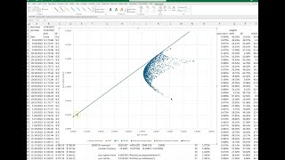
and then what i want to do i'm going to go to data what-if analysis data table and the trick here is i'm just going to click on an empty cell i'm going to put this in column i'm going to click on an empty cell and go okay and it's going and doing all those calculations 10 000 times it's gonna take a second okay so there there's our calculations let me copy that format okay so every time you hit f9 it's going to recalculate that 10 000 times so what it's doing is changing it's changing these weights down here 10 000 times and uh recalculating all those so those would be very easy to graph now so let me highlight these and then we'll go uh insert and let me scroll back up the top because we don't wanna we don't want our chart down here in the bottom we're gonna insert a scatter plot and now we have a really nice graph so this is uh we could say this is the efficient inefficient frontier and let's make these little dots smaller so i'm going to go there i'm going to format the data series under marker uh let's go ahead and move all built in we'll make something that's not so bright and make it as small as possible okay so there we have that and uh get rid of this and what we can do um we have a lot of space this way wasted here like this only goes up to 0. 8 percent because remember our minimum variance portfolio is 0. 86 so really i go like 0.

85 percent and that's my lowest here so i'm going to go here and click i'm going to right click i'm going to go format access and we'll make this point uh zero zero eight five so we can see it a little bit better in that direction okay and then let's just go ahead and label something so i'm gonna go add chart element access title primary horizontal we'll call that standard called portfolio standard deviation and then we'll have to add the vertical title we'll call that portfolio return portfolio expected return okay so so now we have a really nice so when you do two stocks or two securities you just have this line that this this this outlines but now we've done a really nice graph showing showing what's going on so there's a lot of areas here where you're not you're not being rational right why why would you pick a point like why would you pick this point when on the same level of risk i could go straight up and get a much higher return right or at that same point i could go straight to the left and i could get a lot for the same return i can get a lot less risk so that's why all along this border that's that's where the efficient that's where you would pick if you're a rational investor if you're just picking from these three and this point here right here the lowest lowest variance that's what we calculated right here when we when we did the when we use the excel to get the minimum variance right this is the weights so that that combination of weights gives you that point right here now as far left as you could go and and if we kind of get click close to that we can see we're pretty close though if i if i just highlight there hover over it oh come on okay so that's point zero five three four and you can see over point zero three point zero five three and point eight seven and this is point zero five five one point eight six so this is a little bit higher return and a little bit more to the left but anyway you can't get that exactly remember this is ten thousand little dots the more dots you would do then the more this would come come in there anyway this is the power of solver though right because solver you know at this at this level like we maximize the sharp ratio well at this level of risk that's probably one of those points along here you know it's probably probably going to be the best return you know wherever wherever it's point one it would be if you go where where point one two three two is and go to the go to the right it would be like one of those points right there right uh anyway so i hope you understand that now you wouldn't be you wouldn't a rational investor wouldn't want to do any of that report any of the portfolios or any of the dots other than from this minimum variance portfolio all the way up to there right now this one here this very last point i might not have plotted it but this very last point here can we get it if i right click add data label so that's 0.