The Math Behind Generative Adversarial Networks Clearly Explained!
86.78k views2614 WordsCopy TextShare
Normalized Nerd
GAN is considered as one of the greatest breakthroughs in the field of Artificial Intelligence. In t...
Video Transcript:
hello people from the future welcome to normalise nerd in this video I'm gonna explain the gang yes the famous generative adversarial networks I know that this is one of those topics if you don't approach it properly then this might feel really intimidating but trust me by the end of this video you will feel very comfortable with gangs now I put a lot of effort in making these videos so if you like my content please subscribe and hit the bell icon let's get started okay the first thing that you need to know is gang is not
a single model it's a combination of two models the first one is a generative model called G and the second one is a discriminative model called D now what the hell are discriminative and generative models well in machine learning we have two main methods for building predictive models the most famous one is the discriminative method well in this case the model learns the conditional probability of the target variable given the input variable most common examples are logistic regression linear regression etc on the other hand in a generative model the model learns the joint probability distribution
of the input variable and the output variable if the model wants to predict something then it uses Bayes theorem and it computes the conditional probability of the target variable given the input variable the most common example is the naive Bayes model the biggest advantage of generative models over discriminative models is that we can use generative model to make new instances of data because in this case we are learning the distribution function of the data itself which is simply not possible using a discriminator in our Gantz we are using this generative model to produce new data
points that is we are producing fake data points using our generator and we are using this discriminator to tell if a given data point is an original one or it has been produced by our generator now these two models work in an adversarial setup that means they compete with each other and eventually both of them gets better and better in their job let me show you the structure of this thing okay so here's the high-level view of our gang this G and D are nothing but multi-layered neural networks and this theta G and theta D
are just the weights okay we are using neural networks here because they can approximate any function we know that from the universal approximation theorem now look at here suppose this is our distribution function of the original data now in reality we can't really draw that or even mathematically compute that because we input images we mean put voices we input videos and they are higher dimensional complex data so this is only for mathematical analysis okay and look at here this is a noise distribution and you can see that this is just the normal distribution I am
taking and I am gonna sample randomly some data from this distribution and we'll feed that to our generator will to get something from the generator we must input something right and we are inputting here noise that means this Z contains no information and after passing this Z to our model generator it will produce something called G of Z now look at that I have described the distribution of the G of Z with the same X that I have written for the earlier data well I am doing this because the domain of our original data is
same as the range of G of Z this is important because we are trying to replicate our original data so just remember the short forms when I say P data this represents the probability distribution of our original data when I say PZ it represents the distribution of the noise and when I say PG it represents the distribution function for the output of our generator and we are going to pass reconstructed data and original data to our discriminator and this will provide us a single number and the single will tell the probability of the input belonging
to the original data so you can see this discriminator is just a simple binary classifier and for the training purpose when you are putting the original data to the discriminator we will say Y is equal to 1 and when we are going to pass reconstructed data we will say the level is 0 and the D will try to maximize the chances of predicting correct classes but G will try to fool D so we can say that G and D are playing a two-player minimax game what the hell is that well a minimax game is just
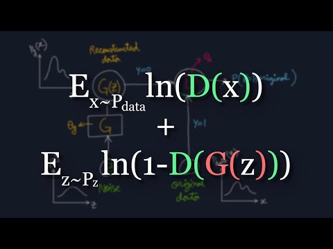
a two-player game like tic-tac-toe where we can interpret the objective as one player is trying to maximize its probability of winning what the other player is trying to minimize the probability of winning of the first player okay now we are saying about maximizing and minimizing but what should they maximize or minimize we need a mathematical expression right and that's called as value function let me show you the value function for this minimax game here well this is the value function for gaen and here mean and Max simply represents that G wants to minimize this expression
and D wants to maximize this expression now I know that at first this might feel gibberish but if you look here closely you will find that this expression is surprisingly similar to the binary cross Centauri function and if you are feeling like that then you are absolutely correct let me show you why so this is our ordinary binary cross interval function for a moment just ignore the negative sign and the summation so this is just the binary kazantip function for one input right why is the ground truth that is the label and Y hat is
just the prediction of the model when y is equal to 1 that is when we are passing the original data the wipe read is equal to D of X so if you just replace these things in the formula you will get lost to Ln of D of X now when we are giving the data as our input the wipe red will be d of G of Z because obviously first we have passed the noise to our generator and it has produced something and then we are giving the produced fake data to the model B and
if you replace these things in the function you will get Ln of 1 minus D of G of Z now let's combine them so I have just added them together and we get this does it look similar to the value function yes but here we are missing the capital E's at the front well they are just expectations understand that this expression is valid for only one data point but we have to do this for the entire training data set right and to represent that mathematically we need to use expectation well expectation is just the average
value of some experiment if you perform this experiment a large number of times suppose you are playing a game where you need to roll a die and your score is the number on the upper face so if you play this game for a really long time then the expected score is 3.5 the formula is very simple you just need to add all the possible outcomes multiplied with their probability so it's kind of a weighted mean so let's apply the expectation on this equation and look at here that we are adding all the scores with their
probability same thing goes for here but this is only true for a discrete distribution if we assume that our P data and PZ are actually continuous distribution then the integral sign will replace the summation and we have to place the DX and DZ accordingly and this whole thing is written in the short form as e ok so now you know the value function for Gann does it look intimidating now I don't think so now I'm gonna tell you how we optimize this function in practice well this is our big training loop and just like every
other neural network we have to optimize the loss function using some stochastic process I am using here the stochastic gradient descent okay so first we enter our big training loop and we fix the learning of G and then we are entering the inner loop for B well this loop will continue for K steps okay and in this loop first we take m data points from the original distribution and M data points from the fake data okay and then we update the parameters of our discriminator by gradient ascent why because remember that our discriminator is trying
to maximize the value function so after we have performed K updates of D we get out of this loop and we fix the learning of D now we are going to train our generator for this case we take only M fake data samples and update the parameters of our generator by gradient descent why because remembers generator is trying to minimize the value function now you might ask why I haven't taken this portion in the update step of generator well look closely does this expression contains any term corresponding to the generator no so the partial derivative
of this term with respect to theta GU will be zero that's why we are taking only this portion one important thing you should note that for every key updates of the discriminator we are updating the generator once okay if you have understood this video so far then you know what is the value function for Gann and how we optimize this in practice but if you are like me and want to know what is the guarantee that our generator will surely replicate the original distribution then take a deep breath and continue watching okay just to be
clear we want to prove that PG will converge to P data if our generator is able to find the global minimum for the value function in other words we want to show that PG is equal to P data at the global minimum of the value function okay this is a two-step process first of all we are fixing the G we wanna see for which value of the discriminator the value function is maximum look here that I have replaced G of Z with X well we can do this because the domain of both of them are
same now if you differentiate this then you will see that the maximum value of this expression will occur if the d of x attains this expression P data over P data plus P G well obviously one can differentiate that and attain this expression but let us look into it ibly so we can represent our value function like this formula a ln x plus b ln 1 minus x and we want to find the value of x for which this expression is maximum so if I take B is equal to 0.6 and a is equal to
0.45 then you will see that the graph looks something like this and the Maxima occurs at point 4 to 9 which is nothing but a Upon A plus B now let's fix the BX as this and replace that into our value function so after fixing D and substituting that in the value function we get this and after a little modification we are getting this long expression and here mimsey just represents that G will try to minimize this thing now understand what we want to do here well we want to prove that probability distribution of generator
will be exactly same as the probability distribution of the data so it makes sense to talk about some of the methods to measure the difference between two distributions and one of the most famous methods are G is divergence that is Jenson Shannon divergence now if you look at the formula for J's divergence then it looks surprisingly close to this long expression isn't it just for a refresher this e here just represents the expectation in the first portion to find the expectation of this value we are using the probabilities from the first distribution but in the
second portion we are using the probabilities from the second distribution okay now let's see if we can somehow get to the J is divergence from this thing okay so after the little modification we are getting this so what have we done here we have just multiplied two in these two logarithms and for this we need to subtract two times the Ln two here all right and if we look closely here then this whole portion is actually equals to two times the J is divergence of P data and PG and obviously we have the negative two
Ln two here so G wants to minimize this what is the minimum value of this expression well the J is divergence between any two distribution cannot be negative the minimum it can get is zero and it will attend zero only when p1 is equal to p2 that is if P data is equal to P G then only this term will be zero and the whole expression will attain its minimum that is minus 2 Ln 2 so voila now you we have proved that add the global minimum of our value function the P G will be
exactly same as P data and our generator is actually trying to attain that state now let me show you how G achieves that state that is different phases of training so at the beginning neither the discriminator nor the generator knows what they are doing so the P G is not replicating the P data and the classifier discriminator is not classifying as well after updating the theta D that is when the discriminator has learned something so the classifier will be better so now the discriminator can actually distinguish between the real data and the fake data now
after the generator has learned something look at that the distribution P G is now closer to the P data and the discriminator is trying to predict the true level of the data points but it is not performing as well now at the end when the generator has attained the minimum of the value function then it has successfully replicated the distribution function of the data point so now PG is indistinguishable from P data so now it is impossible for the discriminator to tell which data point is an original one and which data point is a generated
one so the discriminator will output 0.5 for every input and that is what we want to achieve well this is a very simplistic view of the gaen in reality training the Gann is really hard the goal of this video was to make you understand Gantz I hope you are now very comfortable with the concept of ganz and if you have understood everything that I have talked about in this video then do congratulate yourself because now you know the math behind one of the finest inventions in AI I hope you have liked this video please share
this video and subscribe to my channel stay safe and thanks for watching [Music]
Related Videos

26:46
Understanding GANs (Generative Adversarial...
DeepBean
4,626 views
12:03
Understand the Math and Theory of GANs in ...
WelcomeAIOverlords
66,935 views

20:18
Why Does Diffusion Work Better than Auto-R...
Algorithmic Simplicity
434,566 views
![[Classic] Generative Adversarial Networks (Paper Explained)](https://img.youtube.com/vi/eyxmSmjmNS0/mqdefault.jpg)
37:04
[Classic] Generative Adversarial Networks ...
Yannic Kilcher
66,035 views
21:21
Generative Adversarial Networks (GANs) - C...
Computerphile
653,992 views

38:11
Diffusion Models From Scratch | Score-Base...
Outlier
24,551 views
21:01
A Friendly Introduction to Generative Adve...
Serrano.Academy
266,819 views

57:45
Visualizing transformers and attention | T...
Grant Sanderson
332,014 views

1:55:54
Ian Goodfellow: Generative Adversarial Net...
Steven Van Vaerenbergh
132,823 views
![Hopfield network: How are memories stored in neural networks? [Nobel Prize in Physics 2024] #SoME2](https://img.youtube.com/vi/piF6D6CQxUw/mqdefault.jpg)
15:14
Hopfield network: How are memories stored ...
Layerwise Lectures
741,705 views

31:25
Introduction to GANs, NIPS 2016 | Ian Good...
Preserve Knowledge
153,996 views

22:22
All Machine Learning Concepts Explained in...
Infinite Codes
78,668 views

10:30
Why Neural Networks can learn (almost) any...
Emergent Garden
1,292,186 views

28:53
GAN Generative Adversarial Network Explain...
Ranjan Sharma
24,648 views
10:31
The U-Net (actually) explained in 10 minutes
rupert ai
137,359 views
33:34
126 - Generative Adversarial Networks (GAN...
DigitalSreeni
85,193 views

13:11
ML Was Hard Until I Learned These 5 Secrets!
Boris Meinardus
358,210 views

20:09
Variational Autoencoders | Generative AI A...
Deepia
54,829 views
24:24
Building our first simple GAN
Aladdin Persson
119,966 views

2:01:24
Build a Generative Adversarial Neural Netw...
Nicholas Renotte
183,814 views