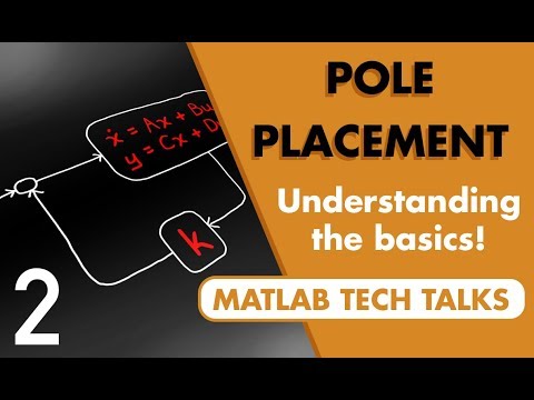
What is Pole Placement (Full State Feedback) | State Space, Part 2
248k views2704 WordsCopy TextShare
MATLAB
Check out the other videos in the series: https://youtube.com/playlist?list=PLn8PRpmsu08podBgFw66-Ia...
Video Transcript:
in this video we're gonna talk about a way to develop a feedback controller for a model that's represented using state space equations and we're gonna do that with a method called pole placement or full state feedback now my experience is that pole placement itself isn't used extensively in industry you might find that you're using other methods like lqr or H infinity more often however pole placement is worth spending some time on because it'll give you a better understanding of the general approach to feedback control using state space equations and it's a stepping stone to getting
to those other methods so I hope you stick around I'm Brian and welcome to a MATLAB Tech Talk to start off we have a plant with inputs u and outputs Y and the goal is to develop a feedback control system that drives the output to some desired value a way you might be familiar with doing this is to compare the output to a reference signal to get the control error then you can develop a controller that uses that error to generate the input signals into the plant with the goal of driving the error to zero
this is the structure of the feedback control system that you would see if you were developing say a PID controller but for pole placement we're gonna approach this problem in a different way rather than feedback the output Y we're gonna feedback the value of every state variable in our state vector now we're gonna claim that we know the value of every state even though it's not necessarily part of the output Y and we'll get to that in a bit but for now assume we have access to all of these values we then take the state
vector and multiply it by a matrix that is made up of a bunch of different gain values and the result is subtracted from a scaled reference signal and this result is fed directly into our plant as the input now you'll notice that there isn't a block here labeled controller like we have in the top block diagram in this feedback structure this whole section is the controller and pole placement is a method by which we can calculate the proper gain matrix to guarantee system stability and the scaling term on the reference is used to ensure that
steady state error performance is acceptable I'll cover both of these in this video but first we need some background information in the last video we introduced the state equation X dot equals ax plus bu and we showed that the dynamics of a linear system are captured in this first part ax the second part is how the system responds to inputs but how the energy in the system is stored and moves is captured by the ax term so you might expect there's something special about the a matrix when it comes to controller design and there is
any feedback controller has to modify the a matrix in order to change the dynamics of the system and this is especially true when it comes to stability the eigen values of the a matrix are the poles of the system and the location of the poles dictates stability of a linear system and that's the key to pole placement generate the required closed-loop stability by moving the poles or the eigenvalues of the closed-loop a matrix now I want to expand a bit more on the relationship between poles and eigenvalues and stability before we go any further because
I think it'll help you understand exactly how pole placement works for this example let's just start with an arbitrary system and focus on the dynamics the a matrix we can rewrite this in non matrix form so it's a little bit easier to see how the state derivatives relate to the states in general each state can change as a function of the other states and that's the case here X dot one changes based on X 2 and X dot two changes based on both X 1 and X 2 and this is perfectly acceptable but it makes
it a little hard to visualize how eigen values are contributing to the overall dynamics so what we can do is transform the a matrix into one that uses a different set of state variables to describe the system this transformation is accomplished using a transform matrix whose columns are the eigenvectors of the a matrix and what we end up with after the transformation is a modified a matrix consisting of the complex eigenvalues along the diagonal and zeros everywhere else now these two models represent the exact same system they have the same eigenvalues and the same dynamics
it's just the sec is described using a set of state variables that change independently of each other when the a matrix is written in diagonal form it's easy to see that what we're left with is a set of first order differential equations where the derivative of each state is only affected by that state and nothing else and here's the cool part the solution to a differential equation like this is in the form Z equals a constant times e to the lambda T where lambda is the eigen value for that given state variable okay let's dive
into this equation a little bit more Z in shows how the state changes over time given some initial condition C or another way of thinking about this is that if you initialize the state with some energy or you add energy from an external input this equation shows how that energy changes and by changing lambda you can affect how the energy is dissipated or in the case of an unstable system how the energy grows so let's go through a few different values of lambda so you can visually see how energy changes based on the location of
the eigenvalue within the complex plane if lambda is a negative real number then this is a stable eigenvalue since the solution is e raised to a negative number and any initial energy will dissipate over time but if it's positive then it's unstable because the energy will just grow over time and if there's a pair of imaginary eigenvalues then the energy in this mode will oscillate since e raised to an imaginary number produces sines and cosines and any combination of the two of real and imaginary numbers will produce a combination of oscillations and exponential energy dissipation
now I know this was all very fast but hopefully it made enough sense that now we can state the problem we're trying to solve if our plant has eigen values that are at undesirable locations in the complex plane then we can use pole placement to move them somewhere else now certainly if they're in the right half plane it's undesirable since they'd be unstable but undesirable could also mean there's oscillations you want to get rid of or maybe just speed up or slow down the dissipation of energy in a particular mode with that behind us we
can now get into how pole placement moves the eigenvalues remember the structure of the controller that we drew at the beginning well this results in an input u equals R kr minus K times X where R kr is the scaled reference which again we'll get to in a bit and K X is the state vector that we're feeding back multiplied by the gain matrix now here's where the magic happens if we plug this control input into our state equation we're the loop and we get the following state equation notice that a and minus BK both
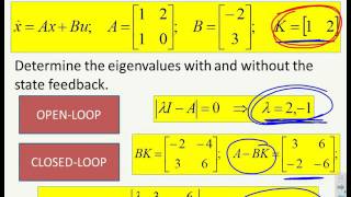
act on the state vector so we can combine them to get a modified a matrix this is the closed loop a matrix and we have the ability to move the eigen values by choosing an appropriate K and this is easy to do by hand for simple systems let's try an example with a second-order system with a single input we can find the eigenvalues by setting the determinant of a minus lambda I to zero and then solve for lambda and there at minus 2 and plus 1 one of the modes will blow up to infinity because
of the presence of the positive real eigenvalue and so the system as a whole is unstable let's use pole placement to design a feedback controller that will stabilize this system by moving the unstable pole to the left half plane our closed-loop a matrix is a minus BK and the gain matrix K is a 1 by 2 since there's one output in two states this results in minus k1 1 minus K 2 2 and minus 1 and we can solve for the eigen values of a CL like we did before and we get this characteristic equation
that's a function of our two gain values now let's say that we want our closed-loop poles at minus 1 and minus 2 in this way the characteristic equation needs to be lambda squared plus 3 times lambda plus 2 equals 0 and at this point it's straightforward to find the appropriate k1 and k2 that make these two equations equal we just set the coefficients equal to each other and solve and we get k1 equals 2 and k2 equals 1 and that's it if we place these two gains in the state feedback path of this system it
will be stabilized with eigenvalues at minus 1 and minus 2 walking through an example by hand I think gives you a good understanding of pole placement and how it works however the math involved starts to become overwhelming for systems that have more than two states the idea is the same just solving the determinant becomes impractical but we can do this exact same thing in MATLAB pretty much a single command I'll show you quickly how to use the place command in MATLAB by recreating the same system that we just did by hand I'll define the four
matrices and then create the open-loop state space object I can check the eigenvalues of the open-loop a matrix just to show you that there is in fact that positive eigen value that causes the system to be unstable and that's no good so let's move the eigenvalues of the system to minus 2 and minus 1 now solving for the gain matrix using pole placement can be done with the place command and we get gain values of 2 & 1 just like we expected now the new closed loop a matrix is a minus BK and just to
double-check this is what ACL looks like and it does have egg in values at minus 1 and minus 2 okay I'll create the closed loop system object and now we can compare the step responses for both the step response to the open loop system is predictably unstable and the step response of the closed loop system looks much better however it's not perfect rather than rising to 1 like we would expect the steady state output is only 0.5 and this is finally where the scaling term comes in on the reference so far we've only been concerned
with stability and have paid little attention to steady-state performance but even addressing this is pretty straightforward if the response of the input is only half of what you would expect why not just double the input and that's pretty much what we do well we're not just doubling it we scale the input by the inverse of the steady-state value in MATLAB we can do this by inverting the DC gain of the system you can see that the DC gain is 0.5 and so the inverse is 2 now we can rebuild our closed-loop system by scaling the
input by K R or by 2 and checking the step response and no surprise it's steady state value is 1 and that's pretty much what there is two basic pole placement we feed back every state variable and multiply them by a gain matrix in such a way that the closed-loop eye ghen values are what we want and then we scale the input to make the steady-state response what we want of course there's more to pole placement than what I could cover in this 12-minute video and I don't want to drag this on too long but
I also don't want to leave this video without addressing a few more interesting things for you to consider so in the interest of time let's blast through these final thoughts lightning-round style are you ready let's go pole placement is like fancy root locus with root locus you have one game that you can adjust that can only move the poles along the locust lines but with pole placement we have a gain matrix that gives us the ability to move the poles anywhere in the complex plane not just along single dimensional lines a two-state pole placement controller
is very similar to a PD controller with PD you feedback the output and generate the derivative within the controller with pole placement you are feeding back the derivative as a state but the results are essentially the same two gains one for a state and one for its derivative ok we can move I can values around but where should we place them the answer to that is a much longer video but here are some things to think about if you have a high order system consider keeping two poles closer to the imaginary axis than the others
so that the system will behave like a common second-order system these are called dominant poles since they are slower and tend to dominate the response of the system keep in mind that if you try to move a bunch of eigenvalues really far left in order to get a super fast response you may find that you don't have the speed or authority in your actuators to generate the necessary response this is because it takes more gain or a more actuator effort to move the eigenvalues from their open-loop starting points full state feedback is a bit of
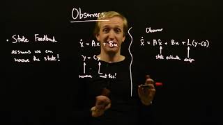
a misnomer you are feeding back every state in your mathematical model but you don't and can't feed back every state in a real system for just one example at some level all mechanical hardware is flexible which means additional states but you may choose to ignore those states in your model and develop your feedback controller assuming a rigid system now the important part is that you feed back all critical states to your design so that your controller will still work on the real Hardware you have to have some kind of access to all of the critical
States in order to feed them back the output Y might include every state in which case you're all set however if this isn't the case you will either need to add more sensors to your system to measure the missing states or use the existing outputs to estimate or observe the states you aren't measuring directly in order to observe your system it will need to be observable and similarly in order to control your system it needs to be controllable we'll talk about both of those concepts in the next video so that's it for now I hope
these final few thoughts helped you understand a little bit more about what it means to do pole placement and how it's part of an overall control architecture if you want some additional information there's a few links in the description that are worth checking out that explain more about using pole placement with MATLAB and if you don't want to miss the next Tech Talk video don't forget to subscribe to this channel also if you want to check out my channel control system lectures I cover more control theory topics there as well thanks for watching and I'll
see you next time
Related Videos

13:30
A Conceptual Approach to Controllability a...
MATLAB
142,292 views
24:34
Easy Pole Placement Method for PID Control...
Aleksandar Haber PhD
3,522 views

14:12
Introduction to State-Space Equations | St...
MATLAB
482,316 views
17:24
What Is Linear Quadratic Regulator (LQR) O...
MATLAB
294,488 views

1:02:51
Introduction to Full State Feedback Control
Christopher Lum
36,838 views
14:25
Pole Placement using State Feedback
richard pates
8,973 views
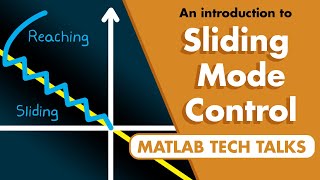
19:33
What Is Sliding Mode Control?
MATLAB
11,292 views

15:44
What Is Feedforward Control? | Control Sys...
MATLAB
161,324 views
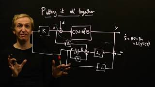
12:55
Control System Design with Observers and S...
richard pates
15,202 views

16:08
Everything You Need to Know About Control ...
MATLAB
559,203 views
13:42
An Introduction to State Observers
richard pates
20,494 views
![Pole Placement for the Inverted Pendulum on a Cart [Control Bootcamp]](https://img.youtube.com/vi/M_jchYsTZvM/mqdefault.jpg)
12:55
Pole Placement for the Inverted Pendulum o...
Steve Brunton
99,333 views

13:57
H Infinity and Mu Synthesis | Robust Contr...
MATLAB
68,804 views

14:41
How 3 Phase Power works: why 3 phases?
The Engineering Mindset
1,324,079 views

11:42
What Is PID Control? | Understanding PID C...
MATLAB
1,823,466 views
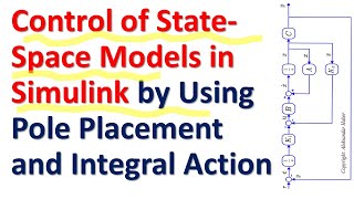
23:38
Simulink Modeling and Control of State Spa...
Aleksandar Haber PhD
2,158 views
8:27
State space feedback 1 - introduction
John Rossiter
62,190 views
14:30
Why the Riccati Equation Is important for ...
MATLAB
26,831 views

17:10
Modeling and Simulation of Advanced Amateu...
Lafayette Systems
71,073 views