Lec 15, Confidence Interval Estimation: Single Population - II
26.18k views2774 WordsCopy TextShare

IIT Roorkee July 2018
Confidence Interval Estimation, Margin of error, Point estimate, Student’s t distribution, Z distrib...
Video Transcript:
[Music] [Music] [Applause] [Music] [Applause] [Music] dear students in the previous class we have predicted the population mean with the help of sample mean where the condition was the Sigma square is unknown now know the Sigma square is known now we will see the next case where Sigma square is unknown then we will see how to predict the population mean for this purpose you have to use student T distributions consider a random sample of n observations with the mean x-bar and standard deviation yes from a normally distributed population with the mean mu then the variable T is nothing but X bar minus mu der by yes daughter by Rho 10 you see that there is a connection between Z Z to be used to write X bar minus mu divided by Sigma by root n but in the T distribution what is happening the Sigma is unknown so we really we are going to use sample standard deviation the other thing is this n should be the smaller number it is less than 30 so when will you go for T distribution when Sigma is unknown when n is less than 30 okay then the variable T equal to X bar minus mu 2 by s by root n follows the student distributions with n minus 1 degrees of freedom now we will see how to predict the conference interval for MU when Sigma Square is unknown if the population standard deviation Sigma is unknown we can substitute the sample standard deviation yes this introduces extra uncertainty since s is variable from sample to sample so we use the T distribution instead of the normal distribution what is the assumption for the T distribution population standard deviation is unknown population is normally distributed with the population is not normal use very large sample the student T distribution the confidence interval is X bar minus P n minus 1 alpha by 2 yes Rutten less than mu less than X bar plus TN minus 1 alpha by 2 yes daughter by root n so this also came from this TN minus 1 alpha by 2 this has come from this expression so when you readjust that this equations then we can get the lower limit upper limit for the population mean so if it is minus X bar minus T n minus 1 alpha by 2 s by root n it is a lower limit if it is a plus X bar plus TN minus 1 alpha by 2 s by root n it is a upper limit so this can be written as like our previous Z distribution X bar plus or minus eme this margin of error so this mu is nothing but T Sigma by root n previously it was Z Sigma by root n now it is T Sigma by root n okay student's t-distribution the t is a family of distributions because for every degree the degrees of freedom you will get you a different T distribution okay the T value depends upon degrees of freedom number of observations that are free to vary after sample mean has been calculated nothing but DS of freedom that is your n minus 1 look at this connection between T distribution and Z distribution we start from the see the flatter one T distributions are Bill shape and symmetric but have flatter tails than the normal so when the degrees of freedom EC initially 5 it is a flatter when the datas of freedom is 13 and so on you see when the degrees of freedom is infinity it is behaving like a Z distribution that is why in many many software packages see there won't be any option for doing Z test there will be option only for doing T test because when the sample size increases for the T test so the behavior of Z distribution T distribution is same then we look at the students of T table you said there is a difference between Z table and T table in Z table whatever value which is given is the area but in a tea table you see that the area is given on the top say point zero five the whatever value which is given inside the tea table is that is a critical value for example if it's alpha by 2 is a point zero five the corresponding T value is two point nine to zero so the body of the table contains T value not probabilities we should be very careful so for example n equal to 3 and degrees of freedom is n minus 1 to alpha equal to 5 then alpha by 2 0. 05 so we are to see where the point 0 4 in the column column line when degree supremest 2 then we can see that is a 2 point 9 to 0 a kind of a comparison between T values and Z values first we will go for this one resume so familiar for us when the confidence level is 95 percentage see the Z value is 1. 96 for different degrees of freedom you see that you see that when the degrees of freedom is 10 it is a 2.
2 to 8 when is it 20 it is 2 point 0 8 6 see that when T equal to 30 the degrees of freedom is 2 point 0 so the value of T approaches Z when n increases you see that initially it is increasing so it is starting you know it is decreasing and finally it reaches 1. 96 this table explains whenever the Daley's of freedom is increases we are getting Z is close to 1 point 9 x 9 6 for the T distribution now we will see how to find out a confidence interval for your T distribution an example is a random sample of n equal to 25 as sample mean is 50 and sample standard deviation is 8 for me a 95% confidence interval for MU the first one is we ought to go for degrees of freedom there are 25 so 25 minus 124 here confidence level is 95 percentage so the significance level is 5% H when they say it is a 5 percentage because it is the upper limit lower limit we have to divide by 2 it is 2. 5 percentage when degrees of freedom is 24 alpha by 2 is point 0 to 5 when you look at the table the T value is 2 point 0 6 so you substitute X bar equal to 50 T equal to 2 point 0 6 yes is 8 and sample size is 25 so you are getting lower limit of forty six point six nine eight upper limit our upper limit or fifty three point three zero two okay I will go to the next category finding the population proportion with the help of sample proportion confidence interval for the population proportion an interval estimate for the population proportion P can be calculated by adding and elements for uncertain uncertainty to the sample proportion that allowance is nothing but e were standard error recall that the distribution of the sample proportion is approximately normal if the sample size is large then standard deviation is your Sigma P Sigma P is root of P Q by n Q is nothing but 1 minus P we will estimate this with the sample data so this is your sample standard deviation we can say standard deviation for sampling proportion root of P Hat 1 minus P hat greater by n okay to find out the lower limit upper limit of the population proportion we have to use the sample values because what will happen we may not know the population P value directly if you know population P value what is the purpose of finding lower limit upper limit we know only the sample proportion so P cap minus Z alpha by 2 root of P cap into 1 minus P cap divided by n less than P Piku plus Z alpha by 2 root of P cap into 1 minus P divided by n so what is happening so with the help of our sampling proportions we can find out this value is a lower limit of our population proportion this value is your upper limit of our sampling proportion you see that we with the help of sampling proportion very able to predict there was a condition but the npq should be greater greater than 5 then only it can be approximated to normal distribution also an example a random sample of 100 people shows that 25 are left-handed for me a 95 percentage confidence interval for the true proportion of left-handers so this problem the P cap is $25 by 100 za is 1.
96 because 95% is confidence level all other P cap is given just you substitute this value and then you put plus decide - you're getting the lower limit of population proportion is 0. 16 5-1 the upper limit of population proportion is 0. 33 for 9 how to interpret this we are 95% confident that the true percentage of left-handers in the population is between 16 point five one percent age and thirty three point four nine for set percentage although the interval from point one six five one to point three three four nine may or may not contain the true proportion 95 percentage of intervals formed from the samples of size hundred in this manner will contain that is more important term another way you can say when you repeat this hundred times 95 times you can capture the true population proportion only 5 times you may not capture true population proportion we'll go to the last one how to predict the population variance so so far what we have seen we have predicted the population mean we have predicted the population proportion now we are going to predict population variance the goal is to for me a conference interval for the population variance Sigma square the conference interval is based on the sample variance so what we are going to do with the help of sample variance we are going to predict the population variance interval we are we are assuming the population is normally distributed we already we have seen that whenever there is a population is there if you take some sample from there when you plot the when you plot the sample variance that will follow Chi square distribution as I told you previously it will be like this okay this will be n minus 1 yes squared or Y Sigma square we are going to use this result when you readjust this right when you readjust this so Sigma Square will be less than or equal to less than or equal to so this will become Chi Square 1 minus 1 this side will become 1 minus 1 es square Chi square n minus 1 here alpha by 2 here 1 minus alpha by 2 so what is happening when you readjust readjust this equation when you readjust this equation for Sigma square you can find out the upper limit and lower limit of population variance yes the same thing the 1 minus alpha percentage confidence interval for the population variance is given by this one you look at this the left hand side is alpha by 2 because what will happen when you look at the chi-square distribution we have given only the right side area when the right shady area is alpha by 2 so what will happen here they will get to a bigger number suppose this was this value is over over 1 minus alpha by 2 so here be a bigger number for example say five he'll be smaller number when you numerator when you divide by bigger number will become smaller value that will become the lower limit of over variance the numerator when you divide by a smaller value it will become bigger number that will become the upper limit of your population variance we'll see you an example you are testing the speed of batch of computer processors you collect the following data sample sizes 17 sample mean is three thousand four sample standard deviation is 74 assume the population is normal determined 95 percentage conference interval for Sigma X bar square here Sigma square is nothing but lower limit upper limit of the sampling variance so n equal to 17 then chi-square distribution has the N minus 1 16 degrees of freedom when alpha equal to point zero five because it is we are finding upper limit lower limit we got two divided by two so point zero two five so when it is alpha by two it is twenty eight point two five so what will happen this is the right side limit when you want to know the left side limit you do in the chi-square table when area equal to one minus 0.
Related Videos

32:33
Lec 16, Hypothesis Testing- I
IIT Roorkee July 2018
52,333 views

24:03
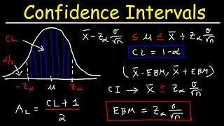
What are confidence intervals? Actually.
zedstatistics
142,012 views
43:39
Confidence Interval For Mean (Large Sample...
PHILOS MasterClass
10,757 views

44:07
Statistics 101: Confidence Interval Estima...
Brandon Foltz
398,273 views

24:37
Lec 13, Distribution of Sample Means, popu...
IIT Roorkee July 2018
40,777 views
20:35
How To Find The Z Score, Confidence Interv...
The Organic Chemistry Tutor
1,081,707 views

29:02
Concept of Confidence Interval and Examples
Dr. Harish Garg
43,651 views
6:44
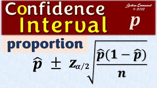
Confidence Interval for a population propo...
Joshua Emmanuel
70,411 views

28:19
Lec 6, Introduction to Probability-I
IIT Roorkee July 2018
98,837 views

14:47
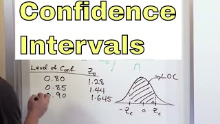
Confidence Intervals In Statistics- Part 1
Krish Naik
142,367 views

1:01:09
Central Limit Theorem - Sampling Distribut...
The Organic Chemistry Tutor
792,965 views

2:24:10
Statistics Lecture 7.2: Finding Confidence...
Professor Leonard
317,429 views

1:18:03
1. Introduction to Statistics
MIT OpenCourseWare
2,029,420 views
21:34
01 - Estimating Population Proportions, Pa...
Math and Science
265,326 views
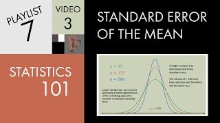
32:03
Statistics 101: Standard Error of the Mean
Brandon Foltz
205,402 views

40:25
Learn Statistical Regression in 40 mins! M...
zedstatistics
231,244 views

4:31
Confidence Interval for a population mean ...
Joshua Emmanuel
608,647 views
11:21
Explaining Confidence Intervals and The Cr...
Very Normal
8,880 views

30:04
ANOVA (Analysis of Variance) Analysis – FU...
Green Belt Academy
90,608 views