Bode Plots by Hand: Poles and Zeros at the Origin
619.2k views1675 WordsCopy TextShare
Brian Douglas
Get the map of control theory: https://www.redbubble.com/shop/ap/55089837
Download eBook on the fund...
Video Transcript:
welcome back to control system lectures this video is a continuation of the series on how to sketch a bod plot by hand we'll build off the last lecture where the transfer function was a constant and describe the bod plot for a transfer function that has either a pole or a zero at the origin if you missed the last lecture you can click on The annotation in the lower corner and it'll open in a new window before we get started I want to just briefly explain what a pole and zero are in the context of a
transfer function if you place the operator s in a transfer function with a value that causes the result to approach Infinity that value of s is called a pole similarly if there's a value of s that causes the transfer function to equal zero then not surprisingly that value is called a zero a pole at the origin means that s equals zero when the transfer function approaches Infinity a transfer function with a single pole at the origin can be written as 1 / s and a transfer function with a single Z at the origin can be
written as just s when s equals z the result of the transfer function is also zero so now let's talk about what the frequency response looks like for a transfer function with a single pole at the origin as we just said the transfer function is 1 / s this transfer function is very important in control systems because it's the llao transform of an integrator but we'll talk more about that later for now we can solve for the frequency response by setting s to J Omega which for our transfer function is -1/ Omega * j a
real quick side note about J J equals the < TK of -1 therefore 1 / J is 1 over the < TK of minus1 if you multiply the top and bottom by the square root of minus1 you can see why 1 / J is just equal to minus J okay back to the problem at hand we found that there is no real component of the result and so we can write that as zero and that the imaginary component is -1/ Omega using this information we can solve for the gain of the transfer function this is
the magnitude of H of J Omega which is positive 1 over Omega and the phase of the transfer function is the argument of H of J Omega and this equals minus 90° to see this graphically you can plot the real and imaginary components on an axxis in our case the real component is zero and the imaginary component is -1 over Omega the length of the vector from the origin to that point is the magnitude which you can see is 1 over Omega and the phase is the angle off the positive real Axis or minus 90°
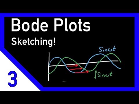
just like we calculated another way to look at this is to draw the block diagram and set the input to the transfer function equal to a pure sine wave of frequency Omega remember that 1 / s is just an integrator so the output is the integral of the sine wave which can be solved easily to be -1 Omega * cosine Omega T you can see that the gain is 1 over Omega and both the negative sign and the cosine contribute to the phase if we look at this in the time domain the input is a
pure sine wave which is this blue line and the output is a negative cosine wave which I'll draw in the same plot so you can see the relationship between the two and you can see that the output which is the green line is lagging behind the blue line by 90° or we say that it has a negative 90° phase shift all three of these techniques produce the same gain in phase for this transfer function but we don't have to do any of that math in the future if we can remember what the frequency response looks
like for a transfer function of this class so let's get to the bod plot already and see what this looks like we've just solved for everything we need to plot the gain and phase at all frequencies on a bod plot remember the vertical axis is in decb which is a log scale and then we also plot the frequencies horizontally on a log scale we calculated before that gain is 1 over Omega so when Omega is 1 radian per second then the gain is also one and when we convert this to decb it becomes zero and
we can plot that point on the gain plot when Omega is 10 radians per second then the gain is 1 over 10 or 0.1 and when we convert that to decb this just equals -2 and we can plot that point on the gain plot and since 1 over Omega is a linear equation we can just draw a straight line between the two points but can we extrapolate that to the next Point by drawing another straight line let's find out when Omega is 100 then gain is 1 over 100 and when we convert that to decb
it equals min-40 DP and so we can see that it is continuing this linear line and we can draw this in either direction for all frequencies the slope of this line is said to be 20 DBS per decade and what that means is for each multiple of 10 the gain drops by 20 DB and on a log scale each multiple of 10 is called a decade drawing the phase for this transfer function is simple since it's just minus 90° at all frequencies so now when you come across the transfer function 1 / s you don't
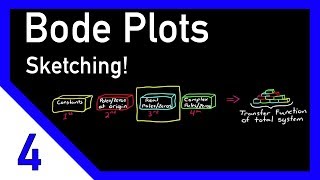
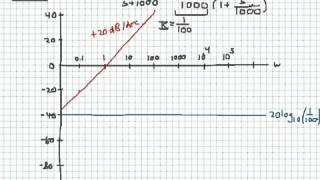
have to do the math you can just draw these gain and phase plots directly but you might be asking right now how often does the transfer function 1 /s arise all by itself what if the function still has a pole at the origin but is slightly more complicated for example 5 / s or 3 / s^2 now how can you draw the Bodi plot directly from this well you can rewrite the first transfer function as a gain of 5 * 1 / s and you can rewrite the second transfer function as a gain of 3
* 1 / s * 1 s and now because of the properties of logarithms we can take the frequency response of each part part individually and add them together on a bod plot to get the frequency response of the entire transfer function and that's one of the main reasons why we plot on a log log scale so that we can take advantage of adding these frequency responses together rather than having to multiply the responses which would be much more difficult so for this second transfer function we can take the response of a gain of three
and the response of 1 over S Plus the response of 1 / s to get the response of 3/ s^2 now from the last video you'll probably remember that the transfer function for a constant of three is just 20 log 10 of 3 and that the phase for a positive constant is just zero for all frequencies and we just learned that 1 / s has a slope of min-2 DB per decade on the gain plot and a phase of- 90° and so since we have two of these 1/ s's we can just duplicate those on
the bod plot so now to get the full response of the system we just add these three lines together and when you do that you'll get another linear line that has a negative slope of 40 DB per decade with a gain added to it of 20 * the log of three and the phase would just be 0 minus 90° - 90° which is- 180° for all Omega so I've spent this whole time talking about a pole but what about a zero at the origin how can we solve for that well luckily we don't have to
go through all this math again we can use the properties of logarithm again and say that s is just equal to 1 / 1 / s and 1 / s is a pole so now we can state that the frequency response for S is just the frequency response of gain one minus the frequency response of a pole the gain of a transfer function of one is just one which is equivalent to Z DB and it also has a phase shift of zero and when you take zero and subtract something from it you just get the
negative of what that something is so we can easily draw the gain of a zero just by drawing the negative of a gain of a pole which is just a reflection about the real axis and we can do the same with phase so phase becomes positive 90° for a zero and something else to think about if you had a pole times a zero which would just be S / s you would expect the transfer function to go to zero and if you sum the responses of both the red line and the green line You'll see
that the gain does go to zero for all Omega and the same applies to frequency so the math works out in addition now you can draw the frequency response for any combination of constants poles and zeros at the origin using this technique without ever having to do the math now in the next lecture I'll explain how to draw the frequency response of real poles and zeros when they're not at the origin
Related Videos
13:38
Bode Plots by Hand: Real Poles or Zeros
Brian Douglas
367,762 views

12:45
Control System Lectures - Bode Plots, Intr...
Brian Douglas
1,251,049 views

Christmas Jazz ☕ Smooth Jazz Coffee Music ...
Sweet Morning Cafe
13:54
Gain and Phase Margins Explained!
Brian Douglas
661,890 views

Cozy Winter Coffee Shop Ambience with Warm...
Relax Jazz Cafe
18:04
Signals and Systems - Bode Plots
UConn HKN
158,375 views
29:55
Control Systems Tutorial: Sketch Nyquist P...
Aleksandar Haber PhD
30,617 views

3:21
Liverpool hit Spurs for SIX to go four cle...
Sky Sports Premier League
1,531,618 views

Music for Work — Limitless Productivity Radio
Chill Music Lab
8:23
Bode Plots by Hand: Real Constants
Brian Douglas
570,459 views

12:21
What's a Tensor?
Dan Fleisch
3,766,530 views

December Jazz: Sweet Jazz & Elegant Bossa ...
Cozy Jazz Music
16:42
Bode magnitude plots: sketching frequency ...
ProfKathleenWage
385,055 views

Crackling Fireplace & Smooth Jazz Instrume...
Relax Jazz Cafe

17:51
Nichols Chart, Nyquist Plot, and Bode Plot...
MATLAB
100,009 views

16:36
Introduction to System Dynamics: Overview
MIT OpenCourseWare
377,437 views

Tranquill Jazz In Lakeside | Living Coffee...
Tranquill Jazz Melody
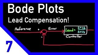
14:19
Designing a Lead Compensator with Bode Plot
Brian Douglas
367,972 views

11:35
Bode Plots by Hand: Complex Poles or Zeros
Brian Douglas
439,819 views
39:10
Sketch Nyquist Plot of Transfer Function B...
Aleksandar Haber PhD
713 views