Lec 8, Probability Distribution - I
64.6k views4361 WordsCopy TextShare

IIT Roorkee July 2018
Probability Distributions, Random variables, Probability density function, cumulative distribution f...
Video Transcript:
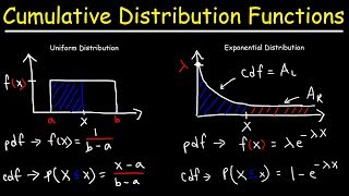
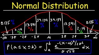
[Music] [Music] [Applause] [Music] [Applause] [Music] good morning students we are entering to the eighth lecture on this course that is a data analytics with the Python today the topic is probability distributions so what we are going to cover today it is very interesting topic we are going to see the some empirical distribution and its properties then discrete distribution in the discrete distribution we are going to see binomial paesan hyper geometric distributions the continuous distribution we are going to see the uniform exponential normal distributions first of all what is distribution what is the purpose of studying the distribution the distributions describes the shape of a batch of numbers there is a meaning of distribution okay suppose the different set of number is there you want to show what shape it follows whether it is a bell-shaped we can call it as a normal distribution if it is forming a rectangular shape we can call it as a uniform distributions like this that describes the shape of your batch of numbers the characteristics of the distribution can sometimes be defined as a small number of numerical descriptors called parameters so each distributions characteristics is expressed with the help of its parameters parameter is nothing but for example normal distribution it has two parameter one is mean and variance with the help of that you can draw the distribution that is a parameter y distribution can serve as a basis for standardized comparison of empirical distributions because if you want to compare with phenomena with your very standard distributions we can come to know that what distribution it follows then it will help you to estimate the confidence intervals for inferential statistics that will see what is the meaning of conference interval in coming classes then for me a basis for more advanced statistical methods for example fit between observed distribution and certain theory called distribution is an assumption of many statistical procedures suppose why we ought to study the distributions suppose if you are doing your simulation for example the arrival pattern follow a Poisson distributions suppose setup data you were collected if you prove that it is arrival follow Poisson distribution already there is a mean and variance in other population parameters already defined it if you're a natural phenomena you are able to compare with this standard distributions there are well-defined distribution parameter is there that parameter you can use as it is that is the purpose of studying the distribution then we will go for what is the random variable if you want to construct a distribution it is the relation between X and corresponding probability X comma P of X so here the X is nothing but random variable a variable which contains the outcome of a chance experiment is the random variable it is a kind of a quantifying the outcome suppose we're tossing a coin for X equal to 1 is getting hit 0 getting tails so 1 is nothing but here random variable so the X the X is the random variable that can take the value of 1 and 0 if the X well is 1 it is a head if the X 1 value 0 it is a tail a variable that it can take on different values in the population according to some random mechanism so the value of 1 and 0 it follow certain mechanism random variable can be a discrete it may be a distinct values countable for example here is a discrete random variable for example mass it is a continuous random variable then probability distributions the probability distribution function our probability density function PDF of a random variable X means the values taken by the random variable and their associated probabilities if you make a relation between X and corresponding probabilities P of X are f of X that if we plot that point that will form your distributions so PDF of your discrete random variable also known as p. m. of probability mass function example let the random variable X be the number of hits obtained in your two tosses of a coin there are two possibility when you toss two times two tosses first toss you may get hit second toss you may get hit then H thing tail telltale so these are the sample space probability density function of a discrete random variable suppose we are tossing a coin two times the probability of getting zero head is 1 by 4 the probability of getting 1 head is 1 by 2 the probability of getting two heads is 1 by 4 some should be 1 C in there in the x-axis the random variable is taken zero in y-axis corresponding probabilities marked so in x-axis random variable in y-axis corresponding probability this is called as the distributions now probability distribution for a random variable X we will do a small numerical problem a probability distribution for you a discrete random variable X is given so X is given corresponding probability distribution is given so this is an empirical distribution suppose if you want to know what is the probability of X less than or equal to 0 so what you have to do wherever random variable X is 0 and less than or equal to 0 you would add add that for example point D 0 plus point 1 7 plus 0.
15 plus point 23 you'll get 0. 65 suppose if you want to know the probability for the random variable - 3 2 1 - 3 less than or equal to X less than or equal to 1 so you have to add minus 3 to 1 point 1 5 plus point 1 7 plus point 2 0 plus 0. 15 when you add it will get 0.
67 how to plot a discrete distributions so number of crisis for example is taken the probability of happening that crisis also given for example the probability of getting zero crisis is zero point three seven four one crisis zero point three one and so on so in x axis you mark the random variable in Y axis you plot the probability right when it is zero point three seven so when it is one one you see that these are discrete these points these points cannot be connected in x axis this random variable has to come into the x axis this probability has to go to y axis for example 0. 37 this one here what will happen you cannot connect this line because it is a discrete because you may have when X equal to one when X equal to 2 when X equal to 1. 5 there is no value if it is a discrete distribution you cannot connect these points that's why it is called discrete distributions okay the requirement for your discrete probability density function the probabilities are between 0 & 1 inclusively the total of all probabilities equal to 1 and sum up probability we have seen that already it is 1 next the term will see cumulative distribution function the cumulative distribution function of a random variable X defined as capital f of X is the graph associating all possible values are in the range of possible values with P of X less than or equal to small X cumulative probability distribution function is just adding the probabilities though CDF always lies between 0 to 1 that is 0 less than or equal to capital f of X should be less than or equal to 1 where capital f of X is CDF cumulative density function then there is a very important property is the expected value of x x be a discrete random variable with the set of possible values of D and pmfs P affects the expected value our mean value of x is denoted s generally expect early effects or new effects is Sigma of X multiplied by P of X so Sigma of X and multiplied by P of X is your expected value of X what is the meaning of this mean and variance of your discrete random variable is look at this there are picture-in-picture be the left side the mean is same for both the distribution but look at the variance the left side figure it's worse there are a lot of variance the right ends figure it is less variance the probability distribution can be viewed as they're viewed as a loading with the mean equal to the balance point so mean is nothing but it's like kind of a balance point over which the distribution lies Part A and Part B illustrate equal means but party illustrates larger variance see the second case mean and variance of discrete random variable the probability distribution listed in parts a and b differ even though they have equal means and equal variances the shape of the distribution is differs now we will see how to find out an expected value use the data below to find out the expected number of credit cards that a a customer to your retail outlet outlet will possess so X is a random variable that is a how many number of credit cards in the customer is having the P of X equal to capital X is corresponding probability so 0 equal to 0 P of X is point 0 8 that means probability of a person having 0 credit card is eight percentage probability of person to have for example 6 credit card is one percentage so how to find out the expected value you have to multiply by X and corresponding probability you have to submit so 0 into point 0 8 plus 1 into 0.
28 plus 2 into 0. 38 and so on plus 6 into point zero one one point nine seven you can make it round 2 that means the the customers they can have an average two credit cards suppose any customer if you take randomly average that customer can have two credit cards here an example of meaning of this what does mean now you'll see how to find out the variance and standard deviation of an empirical distribution previously we have seen mean X into P Sigma of X and D P of X now we will see how to find out the variance of your empirical distribution let X have the p. m.
of P of X and the expected value is mu we know already the mean of your empirical distribution now we have to find out the variance of the empirical distribution then the variance of X denoted is V of X our Sigma square X or Sigma square the variance of X is equal to Sigma of X minus mu whole square into P of X variance can be written as e of X minus mu whole square the standard deviation is just square root of this we will see you an example a quiz scores for a particular student are given below 20 25 and so on find the variance and standard deviation so before knowing the standard deviation first you have to find out the mean because the mean is required so that mean if you add and divide by corresponding elements number of elements will get 21 okay for example first we will construct a frequency distribution you see 12 is repeated by one time 18 is repeated by two times 20 is repeated by 4 times 25 or exam 25 is repeated by 3 times then we have to find the probability the probability is nothing but there the relative frequency as I told you one definition of probability is relative frequency so what is the what is the cumulative frequency here first you have to find out total frequency 1 + 2 3 3 + 4 7 8 10 13 there is a cumulative frequency so the probability here we are obtaining by by using the concept of relative frequency so the relative frequencies we are adding all the frequency that is a total so wonder by corresponding sum of all frequencies to it'll be sum of frequencies now the MU we can find out mu in another way also we know that already we are done know this relative frequency is Sigma of EF in diameter by Sigma F how to find out the mean sigma of expected value x + D P of X 12 Li into point 0 8 + 18 into 0. 15 plus 20 into 0. 3 1 + 22 into point zero 8 Sigma of X and D P of X that is 21 one way you can add all the values you consider by number of elements otherwise from this empirical distribution what is X is given X is 4 12 18 12 probability is given so if you want to know the mean X and T P of X now we are going to find out the variance so P 1 here is point 0 8 X 1 is 12 minus mu whole square plus P 2 is 0.
15 X 2 is 18 minus mu whole square and so on when you add it you will get the variance and the when you take square root of will get D ya you see that and going back point zero eight so 12 minus 21 whole square plus 0. 15 18 - 21 whole square plus 0. 3 1 20 - 21 a whole square when we simplify the variance is thirteen point two five standard deviation is three point six four so what do I have then seen this problem the data is given first we constructed here empirical distributions then we use the formula of mean and variance to find out the mean and variance the other shortcut formula to find the variances is nothing but the e of X minus mu whole square for example already we have seen Yi of X minus mu whole square when you square it and simplify it you will get this formula so variance of X equal to Sigma square Sigma of X square minus P of X minus mu square this can be written as e of X square minus G of X whole square just you have to expand it will get this answer so let us find out the mean of your discrete distribution the formula for finding the mean mu equal to expected value of X that is X into P of X so X is given P of X is given multiply X and D P of X after doing that when you sum the sum is 1 so the mean of this empirical distribution is 1 let us find out the variance and standard deviation of this empirical distribution there is a discrete distribution so Sigma square we know X minus mu whole square into P of X so X is given P of X is given first to find out X minus mu then X minus mu whole square then multiply this X minus mu square by P of X and submit we are getting 1.
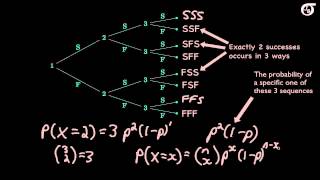
2 so the variance is 1. 2 you take square root the standard deviation is 1 point 1 0 okay suppose then another distribution say X is given P of X is given X into P of X so when you plot it the mean you see that the mean need not be exactly 1 or 2 or 3 mean value may in between 1 & 2 so mean value need not be discreet only the random variable is discrete here some of the very important properties of expected values suppose the expected value of a constant is constant only when you want to multiply two random variable Y of X plus y we can write e of X plus e FY e of X given Y is not division it is a conditional it is a kind of a conditional probability so e of X given Y need not be will not be equal to a of X to order by a of Y and same thing Yi of XY is not equal to e of X modeled by Fi unless they are independent if they are independent we can write e of XY equal to a of X and B of Y otherwise you cannot written so if a random variable come along with the constant that constant can be removed out of this expected value for example Y of ax the ei can be brought left side so a ye of X here where the a is the constant so you see that it is informal a of ax plus B that a can be brought up side so ye of X then we knew expected value of B constant is the constant itself which will become a yeah of X plus B where a and B are constant then properties of variance so variance of a constant is 0 if x and y are two independent random variable then variance of x plus y equal to variance of x plus variance of y variance of x minus y equal to variance of x plus variance of y it should be very careful here suppose there are two group is there Group one and group two if we want to know the difference in the variance you have to add their variance if be a constant then variants of B plus ax because variants of B will become 0 it will become only variance of X if a is a constant then variance of AX is because variance it is quiet term and you bring left side of the bracket they would write es square and variance of X there our proof is therefore this if a and B are constant then variants of AX plus B equal to a square variance X then variance of B will become 0 then answer is a square variance of x if x and y are two independent very random variable and a and B are constant then variants of ax plus B y equal to variance s squared variant ax plus B square variance Y then covariance for two discrete random variable x and y e of X equal to MU X and EF y equal to MU Y then covariance between x and y is the defenders covariance of x comma XY equal to can be written as sigma XY e of x minus mu x and e of y minus mu y when you simplify you look at D of XY minus mu X multiplied by me why there is a covariance in general the covariance between two random variable can be positive or negative if random variable move in the same direction then the covariance will be positive if the if they move in the opposite direction the covariance will be negative properties of covariance if x and y are independent random variable their covariance is 0 since Y of XY equal to EF x nu i if it's independent covariance there won't be any variance covariance of x axis variance of x similarly covariance of YY is simply variance of Y then correlation coefficient the covariance tells the sign but not the magnitude about how strongly the variables are positively are negatively related the correlation coefficient provides such measures of how strongly the variables are related to each other so the covariance is only giving the direction not the magnitude but the correlation is giving the magnitude for two random variable x and y EF x equal to me of x and e fi equal to MU y the correlation coefficient is defined as covariance of XY donor by Sigma X Sigma Y these students now we are going to some special distributions we will study some special distribution in discrete category and continuous category the discrete we'll study about the binomial distribution and Poisson distribution and hypergeometric distribution in a continuous car degree because we are going to study uniform exponential and normal in this class I will explain the theory and corresponding it's a parameters outer end of this class we'll use Python to find out various parameters varies mean and variance of your distributions and corresponding probabilities in the the practical class first one is the binomial distribution let us consider an example to explain the concept of binomial distribution let us consider the purchase decision of your next three customers who enter a store there are three customers going to enter their store and the basis of past experience the store manager estimates that the probability that any one customer will make a purchase is 0. 3 0 what is the probability the two of the next three customers will make the purchase now look at this the tree diagram the first customer there is a two possibility yes is the purchase EF is no purchase X is the number of customers making purchase so you'll see that is the end here now what is happening the first customer he can purchase or not purchase second customer different possibilities third customer different possibilities now we look at the experimental outcome this this possibility look at this possibility success success success look at this possibility success success failures look at this possibility success failure success then success failure failure failure success success failure success failure failure failure success failure failure failure so we have written all possibilities now the question is out of three customers what is the probability that two customers will make a purchase what is the meaning SS is all three customers have purchased so value of x equal to three random variable second case two customer have purchased third customer did not buy so he exits two because here the XS the number of customers making purchase the first possibility X equal to three the second possibility is two third possibility to the fourth possibility is one two one one zero now the question is what is the probability that three two out of three customers will make a purchase you see that there is a possibility the first customer it's a possibility SSE F s FS emphasis what is the probability of success is P P and 1 minus P we know P is 0.
3 so 0. 3 square 0. 7 negative points 0 6 3 4 second category also we are getting P first is success P failure 1 minus P again success is P so P Square material by 1 minus P so 0.
Related Videos

29:34
Lec 9, Probability Distribution - II
IIT Roorkee July 2018
49,924 views
31:15
But what is the Central Limit Theorem?
3Blue1Brown
3,448,953 views

7:03
Are you Bayesian or Frequentist?
Cassie Kozyrkov
246,203 views
16:17
Probability Distribution Functions (PMF, P...
zedstatistics
1,100,517 views
20:27
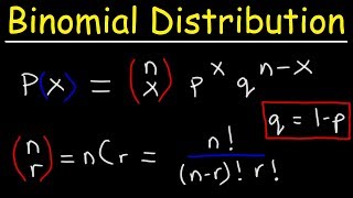
Finding The Probability of a Binomial Dist...
The Organic Chemistry Tutor
1,808,227 views

29:14
Lec 7, Introduction to Probability-II
IIT Roorkee July 2018
65,893 views

9:12
Internet is going wild over this problem
MindYourDecisions
134,485 views
10:48
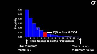
An Introduction to the Geometric Distribution
jbstatistics
313,143 views

16:20
Probability Distribution Functions - PMF, ...
Confidence Matrix
123,614 views

14:24
Poisson Distribution EXPLAINED in UNDER 15...
zedstatistics
306,892 views

2:09:55
Session 40 - Probability Distribution Func...
CampusX
61,535 views
11:02
Cumulative Distribution Functions and Prob...
The Organic Chemistry Tutor
619,929 views
29:30
Normal Distribution & Probability Problems
The Organic Chemistry Tutor
1,200,610 views

10:30
Why The Sun is Bigger Than You Think
StarTalk
290,373 views

1:18:03
1. Introduction to Statistics
MIT OpenCourseWare
2,029,420 views

40:25
Learn Statistical Regression in 40 mins! M...
zedstatistics
231,238 views
27:25
Convolutions | Why X+Y in probability is a...
3Blue1Brown
671,046 views

8:37
Why Technocracies are Increasingly Popular...
TLDR News EU
71,772 views
14:11
An Introduction to the Binomial Distribution
jbstatistics
726,161 views