Bode Plots by Hand: Real Constants
570.46k views1509 WordsCopy TextShare
Brian Douglas
Get the map of control theory: https://www.redbubble.com/shop/ap/55089837
Download eBook on the fund...
Video Transcript:
welcome back to control system lectures just to let you know I've decided to drop the prefix on the video titles because they were taking up too much real estate but these videos are in the same series of lectures so if you're subscribed to control lectures you'll still receive these Updates this video is a continuation of the introduction to Bodie plots that I posted last week and here I'll discuss how to sketch a bod plot by hand directly from the transfer function and this first video will only cover when the transfer function is a constant gain
now you might be asking yourself why do we need to learn how to sketch Bodie plots by hand when we have computer programs such as mat lab that can generate a b plot with a touch of a button I've been a controls engineer for over 10 years now and to be honest I very rarely ever had to sketch a b plop by hand but while you might never actually need to do this there are still at least two compelling reasons to learn this skill the first is that by practicing this it gives you an intuitive
understanding of how poles and zer affect the frequency response of a system without having to actually ever plot the response and the second is that it gives you the ability to estimate the transfer function just by looking at the frequency response of a system and this is particularly handy when you're trying to estimate a transfer function say from the output of a frequency sweep on a new structure that you're building so Recall now from the introduction to the bod plot video that when you have a transfer function h of s you can calculate the steady
state frequency response by setting s to J Omega then you can solve for the real component and the imaginary component and rewrite h of J omega as just the real component plus the imaginary component uh times J if we were to plot this on a real an imaginary axis where the real component is just drawn on the horizontal line and the imaginary component is drawn on the vertical line the gain of the transfer function for that particular frequency is just the length of the line from the origin to that point on the real imaginary axis
that can be written as the square root of the real part squared plus the imaginary part squared or in shorthand notation you can just put these two vertical lines around it which means the magnitude of H of J Omega and the phase is just the angle of the vector off the positive real line and we can write this as the arct tangent 2 of the imaginary part and the real part and in shorthand notation you can just write this as the argument of H of J Omega we can establish the sign of the phase by
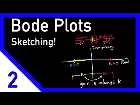
which side of the real line it appears on in this case it might be about 45° if we continue it a little bit further it might be 120° but if we go down below the real line then it becomes negative so -60° in that case so let's revie you the simplest transfer function there is which is a constant and see how that is represented on a Bodi plot in this case the transfer function h of s is just equal to K which can be any real number either positive or negative and we can represent this
in block diagram form by showing that the input gets multiplied by K and becomes the output or U of S is the input and Y of s is the output now we can apply the gain equation from above which is the magnitude of H of J Omega to this constant K which is just the magnitude of K which is a positive K and the phase which is the argument of H of J Omega is equal to the arc tangent 2 of the imaginary part which in our case is zero and the real part which is
K and again K can be either positive or negative and that's why we're using AR tangent 2 to keep track of the sign let me explain it this way if we were to plot this on the real and imaginary axis then all of the values would lie on the real line since there is no imaginary component if K is a positive number then it'll appear on the right side and if it's a negative number it'll appear on the left side but one thing to note about both of these positions is that whether K is positive
or negative the point still exists exactly a k distance from the origin and since gain is the distance from the origin the gain is always k for constants whether they're positive or negative phase on the other hand is different for the first value a positive K phases 0 de but for a negative K it's 180° off the positive real line traditionally we would just say minus 180° but they're equivalent so if the constant is positive then the phase is 0 degrees and if the constant is negative then it's minus 180° and that's why I like
to use arc tangent 2 because it keeps track of the sign of K for you so you don't have to think about that if you just use arc tangent you'd have to remember to subtract 180 in certain cases and not in others but I'd prefer not to remember that and just use arc tangent to so now that we have our gain in Phase how can we represent this on a bod plot well the gain is easy like we said before it's just k for all frequencies but to plot it on a Bodi plot we have
to converted into decb which is just 20 * the log base 10 of the magnitude of K and again it's constant for all frequencies so it's just a horizontal straight line and luckily for this example phase isn't much more difficult phase is 0 degrees when K is positive and it's Min - 180° when K is negative but again the phase stays constant either at 0 degrees or at minus 180° it stays constant across all frequencies so if it's it's not too intuitive looking at this at a bod plot or on a real and imaginary axis
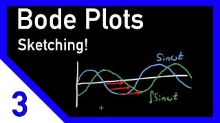
another way to think about this is just input a sign wave through the block diagram a sine wave input produces a sine wve output whose amplitude has been adjusted by a factor of K also if the input was a positive sine wave and the K was a Nega one the output would just be flipped along the vertical axis like this of course as you can see this is just a phase shift of 180° so let's do one last example and this is with a very simple electrical circuit let's say you had a voltage generator whose
output was a sine wave and the positive voltage was then applied to a resistor and both of them were tied to ground the resistor has resistance r a current would be induced I and using ohms law we know that V equals IR but if we wrote this as voltage changed over time it would be V of time equal I of time * R since resistance wouldn't be changing we could take the LL transform of this equation and then solve for the output I over the input V and get 1 / R which is the transfer
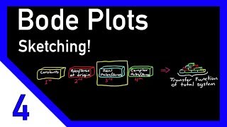
function for this simple circuit and since the resistance isn't changing with Time 1 / R is just a constant and we could represent this on a Bodi plot as a constant gain at 1 / r with a phase shift of 0 degrees I know it's 0 degrees because R is going to always be positive so this is what the B plot would look like for a very simple constant transfer function of course most transfer functions aren't this simple they can be made up of any number of complex or real poles and zeros but the step-by-step
example here of how we go about generating a bod plot still holds up for those other parts and so what I'll do in the next couple videos is expand on all those different types of transfer functions and then show you how to approximate them very easily using just a few simple Concepts and since the next few videos all tie together nicely I'm not going to wait a week to put them out I'll try to get most of them out over the next couple days so if you don't want to miss anything on how to sketch
B plots don't forget to subscribe thanks for watching
Related Videos
8:59
Bode Plots by Hand: Poles and Zeros at the...
Brian Douglas
619,191 views

12:45
Control System Lectures - Bode Plots, Intr...
Brian Douglas
1,251,049 views

BEAUTIFUL CHRISTMAS MUSIC 2025🔥 Relaxing ...
Autumn Melody

16:08
Everything You Need to Know About Control ...
MATLAB
586,849 views

December Jazz: Sweet Jazz & Elegant Bossa ...
Cozy Jazz Music
13:54
Gain and Phase Margins Explained!
Brian Douglas
661,890 views

Instrumental Christmas Music with Fireplac...
OCB Relax Music
13:38
Bode Plots by Hand: Real Poles or Zeros
Brian Douglas
367,758 views
14:19
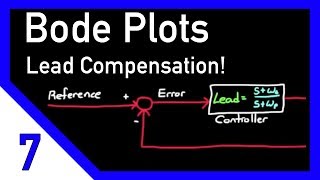
Designing a Lead Compensator with Bode Plot
Brian Douglas
367,972 views

11:35
Bode Plots by Hand: Complex Poles or Zeros
Brian Douglas
439,819 views
13:53
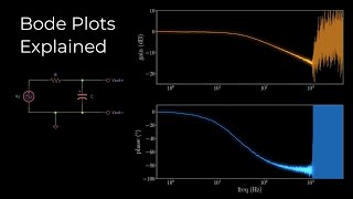
Bode Plots Explained
Curio Res
50,715 views

24/7 Christmas Fireplace Music 🔥 Relaxing...
Cozy Cottage

Jazz & Work☕Relaxed Mood with Soft Jazz In...
Jazz For Soul
20:22
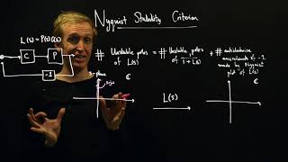
The Nyquist Stability Criterion
richard pates
12,110 views
11:27
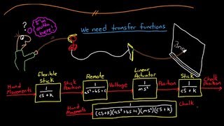
Control Systems Lectures - Transfer Functions
Brian Douglas
703,458 views

Classical Christmas Music & Fireplace 24/7...
Odd Eagle

13:10
The Root Locus Method - Introduction
Brian Douglas
1,074,843 views

Tranquill Jazz In Lakeside | Living Coffee...
Tranquill Jazz Melody

Celtic Christmas Carols, Instrumental Trad...
Open Road Folk Music
16:42
Bode magnitude plots: sketching frequency ...
ProfKathleenWage
385,052 views