Lec 13, Distribution of Sample Means, population, and variance
40.78k views3427 WordsCopy TextShare

IIT Roorkee July 2018
Distribution of sample, proportion, mean, variance, confidence interval, level of significance, samp...
Video Transcript:
Welcome Students, last class we have started various sampling distributions. We have seen the sampling distribution of mean. In this class, we will continue from the sampling distribution of mean then we will talk about the sampling distribution of proportions and sampling ddistribution of the variance.
Then I will introduce the concept of chi-squared distribution. We will do some problems then with that we can close this lecture. Before going to this lecture just to recollect what we have done in the previous class.
This is a population from the population I am taking a sample 1, say, sample 2, sample 3, sample 4. For each sample I can find out the sample mean and sample variance for example if I write x1 bar this is for sample 1 its corresponding mean, if I say, s12 it is the sample with sample variance. So what will you do this is for continuous variable.
Continuous variable in the sense if I am measuring some length or height or something, suppose if I take the same sample assume that I am taking a discrete variable or the categorical variable, categorical, categorical variable in the sense, it can have only two values positive negative or good or bad. Suppose I am taking so this is sample one out of the sample 1,e how many good product is there. So, what is the proportion so then I can call it this is P 1, P 1, another sample that will be P 2 another sample that is P 3.
So, if I plot this P1, P2, P3 directly I cannot plot it. First I have to construct a frequency distribution then, I have to plot it I will get another distribution that is the sampling distribution of proportion. So, there are three point here one is first you take the sample, you take the sample mean, if I plot that sample mean that will follow a normal distribution.
So, mean of the sampling distribution is Mu x bar equal to Mu the variance of sampling distribution is I am writing x bar that is Sigma by root n. This is my first result. What is the first result?
From the population I have taken the sample, if I plot that sample, we will mean that will follow normal distribution. Similarly, in this lecture, what you are going to do, we are going to take some sample from the population, each population is you know, each sample is going, we are going to find out the proportion so proportion means the probability. So I make it P1, P2, P3 that also will follow normal distribution okay.
The third one, which we are going to see in the class, so, we have taken the mean, if you take the variance of each sample, if I plot that variance, if I plot that variance which has come from normal distribution that will follow a special shape, this is called chi-square distribution okay. This is going to be summary of our class. We will continue yeah.
Before that from the previous class we have seen sampling distribution of the mean, with the help of sampling distribution of the mean, we can find out the lower, upper limit of a sample mean that is done with the help of mu plus or minus Z alpha by 2 Sigma X bar. We will see how it is Goal: Determine a range within which the sample means are likely to occur given a population mean and variance. So, what they are asking?
Population mean is given, population variance is given, we have to find out the range of sample means that is X bar, lower limit, upper limit. By the central limit theorem, we know that the distribution of X is approximately normal, if n is large enough with a mean Mu and standard deviation. Let Z alpha by 2 be the Z value that leaves area alpha by 2, in the upper tail of the normal distribution, that is in the interval minus Z alpha by 2 plus Z alpha by 2 encloses probability 1 minus alpha.
So we can find out the upper limit, the upper limit is Mu plus Z alpha by 2 Sigma X bar. The lower limit is Mu minus Z alpha by 2 X bar actually this has come from this formula very, very famous x bar minus Mu by Sigma by root n. From this relationship we can say Mu if you re-adjust that you will get this equation okay.
So, if you get you know you from this you can find out the X bar. So, this value is X bar value we can get the upper limit and lower limit of X bar is a sample mean okay. This was what we have started in the last class.
So, sampling distribution there are three things which you are going to see. One is sampling distribution of sample mean which I have seen. This class, we are going to see the sampling distribution of sample proportion and sampling distribution of sample variance.
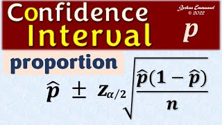
First you will see sampling distribution of sample proportion. P equal to the proportion of populations having some characteristics, we can call it as P is the population proportion. This sample proportion we are going to call it as a small p hat.
It provides an estimate of P. What is the meaning of this estimate of P is sampling distribution of sample proportion. We are going to use capital P, the proportion of population having some characteristics.
Then, sample proportion we are going to call it as P hat provides an estimate of capital P. so, what is the meaning of this one is, with the help of sample proportion we can find out the estimate of population proportion. So, here how the sample proposed is found equal to X divided by n ,X is number of items in the samples sample having the characteristics of interest divided by n is sample size the range of sample proportion is as usual zero less than equal to P hat less than equal to1.
P has the binomial distribution, but can be approximated by a normal distribution when n P Q is greater than 5. Here, Q is nothing but 1 minus P so here it is following binomial distribution. As we know the binomial distribution having properties of having only two alternatives that is good are defective, pass or fail, yes or no.
So, only two alternatives is there okay. So what will you do? From the population, we will take sampling proportion so, when you plot the sampling proportion that will follow a normal distribution.
So, what will happen? This picture shows the different sample as taken from the population for each sample we find out the sampling proportion, if you plot that sampling proportion that will follow a normal distribution. When we know that it is following normal distribution will has two parameters.
So, mean of that sampling proportion is that is the expected value of your P hat is nothing but P the population proportion. And the variance of this sampling distribution is PQ / n that is a P. (1-P) / n.
Actually this need not remember this formula we can derive it because we know, we have seen in the previous class, the mean of binomial distribution is nP, the variance of binomial distribution is nPQ. Actually we have to use capital P for the population so we will, I use capital P. Otherwise we can write 1- P.
Suppose what happen there is a population I am taking proportion 1, proportion 2, proportion 3, proportion 4, like that I may get say P1 hat, P2 hat, I will get too many such proportion. If I plot this, if I plot this sampling proportion that will follow, normal distribution so, we have to find out what is the mean of this sampling proportion distribution. Similarly, what is the variance of this sampling proportion distribution?
We know that since we have taken n sample from the population so the MU P bar equal to Mu X / n okay. We know that not Mu not X bar mu X mu X all know mu X we can write it as n P /n so that is nothing but your population P. So, what this result says that the mean of the sampling proportion is equal to population proportion.
Similarly, according to central limit theorem, this is Sigma by now when you square into Sigma square by n Sigma square by n, so, if you substitute Sigma square is nP I am writing 1 minus P divided by n this is n square. So, variance is because Sigma square by n. So, the Z value for the proportion is so small P cap minus capital P divided by Sigma P we know that Sigma P is root of P into 1 minus P divided by n so P minus so it P minus capital P here capital P represents the population proportion, small P hat represents the sample proportion.
We do one small problem. If the two proportion of voters who support proposition A is P equal to 0. 4, what is the probability that a sample of size 200 yields, a sample proportion between 0.
40 to 0. 45? What is asked here is the population proportion is given that is a 0.
4 that is a 40Percentage. What is the probability that the sample proportion will lie between 0. 4 and 0.
45. So, n is taken equal to 0. 4 and n equal to 200 what is the probability of P(0.
4 less than equal to p^ less than equal to 0. 45) here p is sampling proportion less than or equal to 0. 45.
First you will find out the Sigma proportion that is the standard deviation of sampling proportion. Sigma P equal to root of P Q by n so P is given 0. 4, 1 minus 0.
42 by 200 we got point 0. 34. We have to convert this 1 Sigma P equal to standard normal distribution by using X minus mu by Sigma P so X is given.
X is 0. 4 minus so we have find out the standard deviation of sampling proportion that is the 0. 3464 so that we will convert into standard normal so that we can refer the table.
So, P(0. 4 less than equal to p^ less than equal to 0. 45) .
P(0. 4) this 0. 4 is X equal to the small p -0.
4 is that capital P divided by 0. 03 because that is this your Sigma P there is nothing but did this form is P hat minus capital P divided by Sigma P. So, P cap that is a lower limit is 0.
4, capital P which is given 0. 4 divided by Sigma p so this portion will get 0 and right hand side see the another upper limit of P cap 1 is 0. 45 minus 0.
42 the divided by 0. 034 we got the P ( 0 less than equal to Z less than equal to 1. 44).
When you look at the table P ( 0 less than equal to Z less than equal to 1. 44). we can get 0.
425. So, will summarize what we have done the, it, was asked what is the, what is the probability sampling proportion to lie between 0. 4 and 0.
45. So, what we are done this 0. 4 we are converting to corresponding Z scale it becomes zero.
This 0. 45, we converted to corresponding Z scale it is 1. 44 then we found this area between Z value is 0 to 1.
44 which we got 0. 4251. So, now we have seen this one we will go to the sampling distribution of sample variance.
Let X1, X2 and Xn be the random sample from a population, the sample variance is sample variance Sigma of X minus X bar Whole Square divided by n minus 1. The square root of the sample variance is called the sample standard deviation. The sample variance is different for different random samples from the same population, because every time you may get different sample variance, okay, very important result which we are going to see.
The sampling distribution of sample variance has the mean population variance. So, what is the meaning in that one is, from the population, you take different sample for that sample you find the sample variance we know of that sample variance is equal to population variance but when you take the from the normal population, if you take some sample, then, you find the sample variance. If you plot that that will follow a particular distribution that shape of this will be like this, right skewed distribution.
That distribution is called chi-square distribution that you will see in the next slide. So, another important result is if the population distribution is normal then there is a relationship between sample variance and population variance. That is that relation is n minus 1 s square divided by Sigma square as a chi-squared distribution with the n minus 1 degrees of freedom.
So this x axis is nothing but n minus 1 s square divided by Sigma square. This is nothing but our chi-square distribution. You may see there is a similarity between, there may be intuitively you can connect with the normal distribution.
For example, we say that we will see in the next slide. For example Z equal to X minus Mu divided by Sigma you take different X 1 X 2 X 3 variable so you will get Sigma of X minus Mu. So, what will happen when you square both side when you square both side for different degrees of freedom, so like that you take different sample different means different X 1, X 2, X 3 so this will become Sigma of X minus Mu whole square divided by Sigma square.
So, the square of Z this is will become a chi square. So, what is nothing but Chi square is nothing but Sigma of X minus Mu whole square. I think you know this formula the variance is Sigma of X minus X bar Whole Square divided by n minus 1, sample variance.
So, this numerator can be replaced by that is Sigma of X minus X bar Whole Square can be replaced by n minus 1 into s square divided by Sigma square. That is nothing but your chi-square distribution. So there is a connection between your Z distribution and chi-square distribution the other thing since it is a squared you see that Z it is normal distribution this way, so chi-square distribution is like this, because you see that we have squared that Z value, so that there will not be negative Z; so Chi square will be always positive.
That is the connection between your Z distribution and Chi-square distribution. What will happen? From the sample, you would have taken the variance when you plot that sample variance that will follow this shape.
So, this x axis is nothing but your chi-square value. So, the chi-squared distribution is your family of distribution depending on the degrees of freedom n-1. So, when the degrees of freedom it is increasing that means if you are started to take more samples from the population, then, you plot that the variance at the end that will follow a normal distribution.
What will happen? Your chi-square distribution if the degrees of freedom has increased, that will follow a normal distribution. What is the chi-square distribution?
From the population, you take some sample, for that sample, you find the variance, like that you take many sample you will find different variance when you plot that variance that will follow this shape. This shape is nothing but the chi-square distribution. What is this chi-square distribution?
This x-axis is (n-1) s2/ Sigma2, okay. Then, another important concept is degrees of freedom because many of the time we will use this concept degrees of freedom, we will see, what is the degrees of freedom? Number of observations that are free to vary after a sample mean has been calculated.
That is the degrees of freedom. Suppose that the mean of 3 numbers is 8, say 8 so x1 equal to 7, x2 equal to 8 what is the value of x3 what will happen? Since already the mean is known to us we can supply any value to x1 any value to x2.
But you cannot give any value to x3 because we have lost one degrees of freedom because already we know, what is the mean of that? So what is the logic here is when n equal to 3 so the degrees of freedom is n -1 = 2 values can be any numbers but the third is not free to vary from given mean. It is like, example like, assume that there are three chair is there we are asking three student to sit there.
The first person who is entering will have three possibilities. That is the three degrees of freedom because three chairs are available. The second person will have two possibilities there is a two degrees of freedom.
The third one but there is only one chair there is no option for that so you are lost one degrees of freedom. There are if there are n values you will have only n minus 1 degrees of freedom just we have introduced what is the chi-square distribution and how it has connection with the normal distribution. We will do a small problem to understand the application of chi-square distribution.
A commercial freezer must hold their selected temperature with a little variation specification called for a standard deviation of no more than 4 degrees that is the variance 16 degree square you should not exceed 16, and the standard deviation 4. For a sample of 14 freezers is to be tested what is the upper limit of the sample variance such that the probability of exceeding this limit given that the population standard deviation is 4 is less than 0. 05.
What is it asking, what is the probability of sample variance that the, the probability of exceeding this limit is less than 0. 05? You will see the next slide what it says exactly.
So, first thing is we have to find out the Chi square value for n minus 1 degrees of freedom. This is a chi-square distribution there are 14 sample is n the degrees of freedom is for 13. 14 minus 1 13, so, the corresponding alpha is equal to 0.
05, is 22. 36. So, what is asked is, if, if the chi is 22.
36 right we know that the P of n minus 1 s square by Sigma is 4 so Sigma squared is 16 if the chi-square value is 22. 36, what is the value of your sample variance that was the question. What is asked the chi-square value is known to us that is 22.
36 when alpha equal to 0. 05 when chi-square value is 22. 36 what is the maximum value of your sample variance.
So, probability of s square greater than k equal to P n minus 1 s square by 16 greater than chi-square 13 equal to 0. 05. So, this value this value, this value, n minus 1 s square by 16 so with this s squared between that is your K.
So, n minus 1 K by 16 equal to 22. 36 and you simplify we are getting 27. 52.
The result is give the sample variance from the sample size of 14 is greater than 27. 52 there is a strong evidence to suggest that the population variance exceeds 16. That is the application of this chi-square distribution.
We will see in detail there are many applications for a chi-square distribution one is test of Independence, another one is good goodness of it that we will see in coming classes. Now we will summarize in this class what we have seen we have introduced what is the sampling distributions described the sampling distribution of sample means for a normal population. Then we have explained what is the central limit theorem, then, we have seen the sampling distribution of mean, then we have seen the sampling distribution of variance, then, we have seen the sampling distribution of proportions.
Then I have introduced the concept of chi-square distribution how it has connection with normal distribution. Then, we have seen application of chi-square distribution. The next class will go to the next topic, Confidence Interval.
We will continue in the next class. Thank you.
Related Videos

26:03
Lec 14: Confidence interval estimation: Si...
IIT Roorkee July 2018
34,576 views

11:06
Sampling Distributions (7.2)
Simple Learning Pro
228,110 views
6:44
Confidence Interval for a population propo...
Joshua Emmanuel
70,411 views

20:08
Why the p-Value fell from Grace: A Deep Di...
DATAtab
108,060 views
19:07
Intro to Standard Z-Score & Normal Distrib...
Math and Science
59,661 views
6:59
How To...Calculate the Confidence Interval...
Eugene O'Loughlin
565,917 views
24:35
01 - Sampling Distributions - Learn Statis...
Math and Science
390,783 views

19:54
How To Know Which Statistical Test To Use ...
Amour Learning
763,025 views

12:50
Statistics made easy ! ! ! Learn about t...
Global Health with Greg Martin
2,091,121 views

42:09
Teach me STATISTICS in half an hour! Serio...
zedstatistics
2,751,282 views

7:40
Confidence Interval for a population mean ...
Joshua Emmanuel
87,772 views
14:22
Calculating the Mean, Variance and Standar...
StatQuest with Josh Starmer
452,760 views

1:08:17
Hypothesis testing (ALL YOU NEED TO KNOW!)
zedstatistics
284,523 views
![Confidence Interval [Simply explained]](https://img.youtube.com/vi/ENnlSlvQHO0/mqdefault.jpg)
5:34
Confidence Interval [Simply explained]
DATAtab
530,924 views
11:47
Measures of Spread: Crash Course Statistic...
CrashCourse
615,517 views
1:18:47
Introduction to Bayesian Statistics - A Be...
Woody Lewenstein
80,475 views

1:18:03
1. Introduction to Statistics
MIT OpenCourseWare
2,029,420 views

29:14
Lec 7, Introduction to Probability-II
IIT Roorkee July 2018
65,892 views

2:24:10
Statistics Lecture 7.2: Finding Confidence...
Professor Leonard
317,429 views