What Is Mathematical Optimization?

in 1987 the new york times front page read breakthrough in problem solving the breakthrough here refers to the invention of the interior points method an efficient algorithm for convex optimization and here you might wonder what is convex optimization and what is so important about it that the headline refers to it as problem solving and what makes the discovery of this new algorithm for solving convex optimization problems so special that it's made the headline of a journal like the new york times if you are asking yourselves these questions you are in luck because this is exactly

the topic of this video series this series is broken into three parts part one is a short introduction to the active field of mathematics that is optimization and some of its applications in part two we will dive deeper into the topic of convex optimization and we will introduce a fascinating related concept that is the principle of duality the third and last part has a more algorithmic component there we will finally have all the necessary ingredients to overview the interior points method for convex optimization [Music] as a bonus if you stick around until the end you

will know what this ocean animation represents and how it relates to the topic of optimization this video series is intended for anyone who is curious about mathematics and its applications it should be accessible to a wide range of audiences since it does not require any specific background beyond basic linear algebra and basic calculus it is suited for math and computer science students who want to know more about optimization [Music] but also researchers or engineers who might have heard of optimization before and want to know what they can gain from it or how they can use

it in their own work or research projects let me point out here that these videos represent my personal take on the topic of convex optimization so it might be a little different from more traditional expositions that you might find elsewhere and it is by no means exhaustive but my goal here is to give a self-contained presentation that is crisp visual and focuses on building intuition without getting bogged down with too much mathematical details which you can always check later if needed and with that being said it's time to grab some coffee because we're about to

get started before we talk about convex optimization let's take a step back and first define optimization what do we mean when we refer to some problem as an optimization problem well you have an optimization problem whenever you are faced with a bunch of options that you can choose from where each option has a cost associated with it and your job is to make the optimal choice or in other words you need to pick the option with the smallest possible cost note that sometimes in optimization there are situations where we want to pick the option which

maximizes some given metric often referred to as a reward rather than minimize the cost without cause of generality we can simply multiply the reward by -1 and convert a maximization problem to a minimization one so for the rest of this video i'm going to follow a cost minimization convention note also that in this toy example there are only 6 options in general however the number of options could be huge or even infinite a typical example where the number of options is infinite is when you try to pick a real number x from the continuum of

all real numbers that minimizes some given function f say differently you try to pick a scalar x that we refer to as a decision variable such that f of x is as small as possible here x is a one-dimensional scale but it could also be multi-dimensional for example x could be a two-dimensional vector x1 x2 a three-dimensional vector x1 x2 x3 etc more formally an optimization problem is given by three ingredients the first ingredient is a set where our decision variable lives often this is simply rn the second ingredient is a cost function f that

we want to minimize this function maps the set where our decision variable lives to r this function is sometimes known as the objective function the third and final ingredients are constraints on the decision variable constraints come in the form of equality constraints and inequality constraints the equality and inequality constraints together define what is known as the feasible set or the set of possibilities where you can pick the decision variable x from to recap optimization problems are often written in this form let us right away see some examples when the cost function f is a linear

function and when the functions h i and gj that define the constraints are linear functions as well then we have what is known as a linear program linear programs are among the problems that we understand the best and as we will see later on it is essential to understand what happens in the simpler and maybe idealistic linear word before we move on to more complicated nonlinear problems [Music] so in the next three minutes or so let us try to build some geometric intuition about linear programs to visualize linear programs geometrically we need to first understand

how to visualize linear functions there are essentially two ways we could go about visualizing a linear function like this one either we represent it with a hyperplane with equation f of x equals zero or with the vector c that is normal to this hyperplane the hyperplane representation is useful for visualizing where the linear function f takes some given value like maybe f of x equals 0 1 or 2. on the other hand the vector representation is useful for understanding the direction that increases or decreases this linear function [Music] for linear cost functions we prefer the

vector representation the reason is that in the absence of constraints and in order to minimize a cost function f what you need to do is simply move along the vector minus c as much as possible easy enough so now let us see how to visualize linear constraints for linear functions that define linear constraints we prefer the hyperplane representation a hyperplane divides the space in three regions a positive half space a negative valve space and a null region or the hyperplane itself now if you think of the whole space where your decision variable lives as this

cube then a linear constraint for example an inequality constraint will cut off a part of the cube and as you add more and more linear constraints more and more parts of the cube are going to be cut off and the region of the space that we are left with is our feasible region moving on an optimization problem that might be familiar to you is linear regression or the least squares problem here we try to model the relationship between inputs a and outputs b and more specifically we try to fit a linear model so our decision

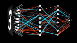
variable is a vector of weight our objective function measures the error in our linear model and note that the objective function is not a linear function but rather a quadratic function and our constraints are well there aren't any constraints in this example there exists quite few variations of this problem for example we could replace the linear model with a more complicated function like a neural network in that case the regression problem becomes a considerably harder problem and this should already give you a hint that some optimization problems are easier to handle than others a third

example of optimization problems i want to show you is portfolio optimization from the field of finance in portfolio optimization you are presented with a list of assets like stocks and your job is to pick which assets and how much of each asset you should buy here your objective is to maximize returns and your constraints are that maybe you have a fixed budget that you cannot exceed and maybe you have a cap on the maximum volatility allowed for your portfolio more generally any problem that involves taking the best decision under constraints is an optimization problem engineering

advertising games are just some examples in conclusion to this first part of this series i would like to point out that so far we have focused on taking a problem and formulating it as an optimization problem we have not yet discussed how you can actually solve these problems in fact optimization problems that have very similar formulations can require a completely different set of techniques to solve and we often need to design specialized machinery for each problem separately in the last couple of decades however something magical has happened we have discovered that a large family of

optimization problems namely convex optimization problems can be solved efficiently in a unified manner once you recognize a given optimization problem as convex then you can apply an already established and mature technology that people have developed for convex problems almost as a black box in the next video we will discuss convexity in more details and see what makes this property so attractive from an optimization point of view and in the third and last video we will peek inside this black box and uncover some fascinating ideas behind it and finally i would like to thank you personally

for making it this far in this video and see you next time