The exercise files for today's course are located in the video description below. Don't forget to like and subscribe. Welcome everyone. I'm Trish Connor Ko and this is Tableau introduction. Tableau is a visual analytics platform that makes it easier for people to explore and manage data and faster to discover and share insights that can change businesses. It helps people and organizations be more datadriven. Tableau supports data prep, analysis, governance, collaboration, and more. This Tableau basic training course is designed as an introduction to Tableau for beginners. On completing the course, students will have a firm grasp of
the basic techniques required to create visualizations and combine them in interactive dashboards. Specifically, students will meet the following learning outcomes, among others. Creating foundational to advanced visualizations working with data in Tableau. Thank you for viewing this Tableau introductory course. Module one covers creating your first visualizations and dashboard. In this module, we'll be getting right to work, diving in head first to Tableau by connecting to an Access database, creating visualizations, and ending with creating a dashboard. Think of this module as a hands-on opportunity to learn how easy it is to get from accessing data to creating
dashboards in Tableau. And we'll fill in all the pertinent details in subsequent modules. So, this module has three lessons. The first lesson is connecting to data in Access. And we're going to use a database named Northwind that is in the files in the video description. So, you might want to go ahead and grab that file and move it somewhere onto your system where you can easily access it. Our second lesson will cover the foundations for building visualizations. And the third lesson will bring everything together in a dashboard. Now, before we get hands-on, there are a
few other things I want to review with you before we get started. And this PowerPoint presentation is in the files in the video description as well for your future reference. So, before we get into Tableau, it's important that you understand the interfaces that you're going to be working in. So, again, you'll have these slides for future reference, and I'll remind you of these things when we get into Tableau. But the first thing I'd like us to take a look at is the data source view. So you'll get to this view once you connect to a
data source. Now the picture on this screen is from an Excel file, right? And you can see that on the left side it is known as the left pane. And at the top of the left pane, it's telling you underneath connections the name of the file and the type of file it is. So this is a sample superstore file that's an Excel file. Because it's an Excel file, it's showing you underneath sheets all of the sheets that are in the worksheets that are in that Excel file. The next thing you'll see is at the top
of the screen. Now, this is when you first go in. This is a blank area. It's called your relationships canvas. It's also known as the logical layer on the canvas. And we'll dive into that a little bit more in a moment. But you're seeing the tables and their relationships in the canvas. If I doubleclick on any of those tables in this canvas, it opens up the joins canvas, which is here, letter C. And we'll talk about that in more details in a little bit. Actually, very shortly once we get into Tableau. On the bottom half
of the screen in the background, you're seeing the data grid. And so when you have your tables up at the top, you can see the data that's in those tables in the data grid. And if you want to explore any metadata, there is also a metadata grid that can be accessed. And I'm pointing to that one now. So that red arrow is pointing to the metadata grid. And then I'll draw another red arrow that's pointing to the data grid. So all of these things aren't open at the same time, but this is just a view
for you to reference when you're working in the application. So I talked about the relationships canvas and the join canvas. Well, this is a further breakdown of that. So the canvas has two layers. The default layer when you go onto the data source page is the relationships canvas and you combine data in that layer using relationships. And then the physical layer which you get by doubleclicking on an object in the logical layer you can use to combine data between tables by using joins and unions. Each logical table contains at least one physical table which you'll
see when we get into Tableau. And again the physical layer is also known as the join canvas or join union canvas. You'll see this when we get into Tableau. And the last slide before we get handson is showing you the breakdown of sheet view in Tableau. So all the way at the top you'll have the workbook name which currently shows book one as you can see in the upper left hand corner there and it's marked with the letter A above it. So it's just saying book one up there. And then the letter B are known
as cards and shells. So this panel here on the left where it's saying pages, filters, so on and so forth, those are cards. And then where it says columns and rows, where you have some of these fields that have been dragged in there and those are shelves. You have a toolbar at the top and that's under your letter C there. So you have a little bit of a toolbar running right underneath your menu bar. And then the letter D is your view. And that's your canvas where you will create a visualization. This area right here.
There is a little button all the way to the left of the toolbar. It's letter E. And that will take you to the start page, the very opening page when you get into Tableau. If you need to get back to that start page, that's the way to do it by using that icon on the far left of the toolbar. Letter F is showing you the sidebar. This is on your left side, right? The sidebar is showing you what you're looking at here. This is the orders table from sample superstore or orders from sample superstore. And
that's what it's saying there. And letter S. And then letter G is at the bottom and that's the data source tab. So if you notice to the right of that we're on sheet one and that's why we're seeing this view. If we want to get back to data source sheet we can or tab we can use that data source tab button there and that will take you back where you can see the grid view and all of that stuff. Underneath all of that the gray band running across the bottom is your status bar. like it's
in pretty much in every other Windows application. You'll find a status bar at the bottom in the gray band and the status bar is just giving you information. And then you have, like I said, we're on sheet one. And to the right of that, you have these little icons that you can create new sheets, new dashboards, new stories. And again, I'll remind you of this when we get hands-on, which we're going to do right now. So now I'm on my desktop and I'm going to show you how to launch Tableau. I'm going to set it
up so it'll be easier access for you going forward. So what I'm going to do is I'm using Windows 11 here. What I'm going to do is I'm going to go to start or I could go to search. I'll go to start cuz this is kind of way cool. And I'm going to just do all apps at the top. And then I'm going to click on the letter A. So it collapses the alphabet. And then I can choose the letter T for Tableau. And when I get to Tableau, I'm not going to click on it.
That will launch it. I'm going to rightclick on it and I'm going to hover over more and I'm going to pin it to my taskbar. So now, if you notice, and I'm going to click away from that. So when my taskbar is displaying at the bottom, the last icon on the right is Tableau. And I'm going to go ahead and click that icon to launch the application. When you launch Tableau, it opens on the home screen where it gives you the ability on the left to connect to a variety of different data sources. So you
can search for data on Tableau server. You can open a file here. You can go to the server to get other types of databases. And then you have when you download Tableau, you get a couple of saved data sources there. One of which is sample superstore, the other is world indicators. On the right side of the screen at the top, you can open a workbook as well from there. And then you have accelerators at the bottom. Accelerators are pre-built dashboards that you can use and you can swap out the data that comes with them with
your data just to give you a jump start if necessary. And you have the ability to access more acceler accelerators on the right side. on the left side. What we're going to do is under the to a file section, we're going to select Microsoft Access and then you're going to browse to wherever you put that Northwind file and you're going to doubleclick it. Now, that Northwind file doesn't require a password. There's no workg groupoup security. So, we can simply just click open. So once you connect to your data, it takes you to data source view.
If you look down at the bottom of your screen, you'll notice that the data source tab is the active tab indicating you're in data source view. In your left pane, you're seeing the name of your database as well as the source. Microsoft Access underneath connections and then instead of seeing sheets like we have in the PowerPoint, you're seeing the tables that are in that database. And if necessary, you can use the add link to add more connections to your data source if necessary. What we're going to do is we're going to start dragging tables. So,
we want to find the orders table in the list in the left pane. Click and hold on it and drag it onto the canvas. And you'll notice quite a few things have changed. So, right now it's letting you know that you're on the orders table from the Northwind database. At the top, it has, if you hover over the orders table instance there, it lets you know that it's a logical table. and that you can doubleclick it to see its physical table. So, let's go ahead and doubleclick orders. And we're just seeing the physical table at
this point. And to go back to our initial view over in the upper right hand corner, you're going to go ahead and click on the X to close the physical layer and get back to the logical layer. It also has in the upper right it defaults to a live connection versus an extract and we'll talk about that in the next module. And then you it says you have zero filters and you can add filters there. We'll talk about that separately as well. So I want to show you what can happen if you drag another table
to this logical level here. Remember this is the relationships canvas. So if I go to drag, look for the order details extended table and drag that onto the canvas. And you'll notice the little noodle line as you're dragging it. It's showing there's a relationship between those tables. But when you let it go, you get this error message. Says the data source uses a connection that doesn't support multiple logical tables. blah blah blah. So instead of reading all of this, I'm going to just close the error message and show you how we're going to get our
other tables in. So it won't let us put them at the logical level. And before we do this, by the way, let's talk about the grid at the bottom. So you're seeing on the left side of the grid, you're seeing a list of all of the fields in the order table in the orders table and their types. Uh the pound sign or hashtag represents a numeric data type and you'll have some dates. It looks like a calendar and then you'll see an ABC which means it's a text data type and you'll see those symbols repeated.
It's showing you all of the information that's in that orders table. At least 48 rows of it here, right? Which is all it has. It's 20 fields and 48 rows. It's telling you right there and you can scroll down to see the rest of your rows and so on and so forth. So now we're going to doubleclick on that orders table in the upper half to get back into the join or union layer. And now I'd like you to take order details extended and drag it there into that canvas. And so now it's showing the
join between the tables and the join represents how the tables are connected to each other. And so in this and you'll learn more details about joins in the next module. But for right now, if you click, if you hover over that join between the two tables up there, it'll say enter join of orders and order details extended. Underneath that, it says order ID equals order ID. So there has to be a common field between the two tables to join them. in an inner join is telling you that it's only showing orders that have extended order
details. If there are orders in there without order details, they will not be showing down in this grid. And now that we've joined the tables like this, if you look in your grid, you'll see that you're getting fields from the orders table, right? And if I scroll across to the right, then you'll see the fields, the matching fields for those particular orders from the order details extended table. So joining actually combines data between two tables. Relationships do not. And you'll learn more about that, like I said, a little bit later on. Go ahead and drag
the customers table and the sales analysis tables into the view. So notice at the top above your orders table it says orders is made of four tables. We have the orders table itself and then we have the related or join tables customers order details extended and sales analysis. So now that we have our tables in, we can go ahead and close the physical layer by again using the X. And you'll notice when we come back to the logical layer, it shows that it's has joined tables. If they're not showing here, that means you need to
doubleclick that to see them. So it's showing you the logical tables on that popup and the physical tables on that popup. And again, you can double click it to see its physical tables. So out here in this view, right, if you notice, something changed. We now have 69 fields and 234 rows because we added other tables. And you can also remember to scroll across to see the other table fields that are in there. And it just goes all the way over to the right. Now, if you want to see more of your data, you can
put your mouse between the upper part of the canvas and your grid on the lower half. Click and hold and you can drag up so you can see more rows of your data. Scroll down. So, now it's showing 100 rows at a time. I can tell that by looking up here in the upper right hand corner. It's telling me that it's showing 100 rows. I can do the right arrow next to it to see the next 100 rows. So on and so forth. I can change the number of rows that it's showing if I want
to. To the right of the rows, you have a gear icon. And if you click on that, it gives you some sorting ability and some other options there. And if you go to the drop-down arrow to the right of that gear, it collapses the grid and then it turns into an up arrow which I can click to expand and show the grid again. Now we're ready to go to sheet view. So right next to your data source tab at the bottom of your screen, go ahead and click on sheet one. And now you're in sheet
view. And just so you know, instead of being called the left pane in sheet view, it's called the sidebar. And you have your data tab at the top. And you also have an analytics tab. Go ahead and click on the analytics tab. Everything is dimmed out right now. We're not going to do any analytic analytics in this module. Go back to the data tab. We will get into analytics later in the course. In that sidebar on the data tab, you have a list of all your tables and all of the fields in every table. And
it also shows you whether it's a text field, whether it's a geographic field, whether it's a numeric field in front of the field name. If you scroll down in that sidebar underneath the sales analysis table and its fields, you'll see measure names. Any numeric field that's in your data source will automatically be converted to a measure in Tableau. So for example, the unit price field from the order details extended table when we use it in our v if we were to use it in a visualization, it would automatically do the sum of the unit price.
So, I'm going to scroll back up to the top and we'll choose the fields that we want for our first visualization here. The first field we're going to use is from the orders table and we're going to drag it to our columns shelf. So, I'm going to use and it's going to be the order date field. So, I'm going to click and hold on order date and I'm going to just drag it up to the columns shelf. right underneath your toolbar. And when I drop it there, a couple of things happened. It automatically puts it
in as just the year of the order date and it starts building the information right here on this canvas. It also selects right now um the recommended it's like a text like a table visualization right now and that pane starts lighting up. The next thing we're going to do, we have our year of order date, and we want the ship state slashprovince to be in our rows. So, ship state/province is also in the orders table. I'm going to click and hold and drag it and drop it in my rows shelf. So, it wants to do
a table here, but I don't want this to be a table. I want it to be a map. Since we have geographical data in it, we can convert it to a map. So, what I'm going to do is in my visualizations panel on the right hand side, I'm going to hover over and you can see I'll point it. I'll do an arrow pointing to the one I want. It's just a plain map. So, I'm going to select that map and it converts the table into a map. And notice now it says longitude generated and latitude
generated. One is in row, one is in columns, but it took out that state province because it converted it so it can be shown as geographical data on the map. So that's what it does there. So on this particular map, we just have the states that have orders basically and they're highlighted. They're shaded on the map. And what we're going to do is up at the top of your map where it says sheet one, you're going to doubleclick that. We want to rename that. So I'm going to just select that sheet name placeholder. It's going
to name it whatever the name of the sheet is initially. I'm going to just type order map and apply. So it changed it there. And I'm going to click okay to cancel that edit title box. And then I'm going to doubleclick on the sheet, sheet one. And I'm going to just name it map. Now we're going to create another sheet and place another viz on it. So to the right of your map sheet tab, you're going to click the plus sign, the first plus sign. It gives you a sheet two. And on this sheet, we're
going to drag order date to the column shelf again. And we don't want the year of the order date for this one. We want the actual date. We're going to do the drop-down arrow. If you hover over that year order date, you'll see a drop-own arrow to its right. We're going to click the drop- down arrow. And in our list here, you'll notice it has year selected, right? What we're going to do is we're going to go down in the list and we're going to select day. So, not in the upper list, but in the
lower list. So, you have year, quarter, month, day, and more. And then you have year, quarter, month, week number, day, and more. In the year, quarter, month, week number. That's the day we want. It's going to actually show the full date, day of order. Well, not the full date, but it's going to show it's they're all in 2006. It's going to show the month and the day, which is what we want. And then what we're going to do is we're going to scroll all the way down on the left. We're looking at our measure name.
So there's a measure named sales under sales analysis and we're going to drag that to rows. And it makes it the sum of sales because it's a measure. So now we have the sum of sales by date. And what we can do is you can hover over any point on your line graph and you can see the day of the order date as well as the amount of sales on that date. We connect it to an access data source. We chose the tables that we wanted and then we went to the first sheet, chose some
fields from the tables and made a map out of it. Now we're on our second sheet and we made a line graph out of the data that we chose. So up at the top where it has the title of the map, we're going to click there where double click where it says sheet two, not the title of the map, the title of the line graph. And we're going to select that sheet name placeholder. And we're going to name it sales amounts by date. And we're going to apply and okay. And then we're going to doubleclick
our sheet 2 tab and we're going to rename that just sales for now. Now that we have two visualizations created, we are going to create a dashboard which allows you to see several views at the same time. So each of these sheets, our map sheet and our sales sheet are two different views. We're going to combine them into a dashboard. So to the right of your sales sheet tab, this time I'm going to have you rightclick on the plus sign and choose new dashboard. And you'll notice on the left side, it just shows the sheets
that are in this file. So, the first thing we're going to do is we're going to just click and hold on the map sheet and drag it into the view. And then we're going to click and hold on the sales sheet and drag that into the view. Now, I want my map to be on the top of the view, and I want my sales amounts by dates to be on the bottom. So, I'm going to hover over the map portion and click on it. At the top, you'll see that little gray band with white lines.
If you put your mouse on that, it changes to a foreheaded arrow. You're going to click and hold and then you're going to just point to the top of the view and it will drop the map at the top and move your line chart to the bottom. Now here we can add filters to our two different viz visualizations rather. I was trying to say vizes and went for visualizations. And the way to do that is for the map. I'm going to hover over the map and you'll see on the right you have the X to
remove it from the dashboard. You have the second icon down is go to the sheet where it resides. Third one is use as filter and the bottom one is more options. So, we're going to click that more options down arrow. We're going to hover over filters and we're going to choose from the list ship state province. And it creates a filter, a visible filter where you're seeing all of the states that are highlighted in the map, all of the states that have sales from our data. And you can use that filter. So, it defaults to
all. I'm gonna go ahead and uncheck all and the entire map disappears. And then I'm going to just check New York. And so it zooms in with New York state highlighted. I'm going to go ahead and check all again. And then for our sales amount as dates visualization, we're going to select it, go to the more options drop- down arrow, hover over filters, and we're going to do day of order date there. So, it gives me the range of order dates. You can see January 15 through June 23rd, 2006. I can click on a date
there or I can use the slider. If I use the slider now, you notice the chart, the line chart updated because now it's showing March 6 through June 23rd. And I'm going to slide it all the way back to January 15th. Now, let's say I wanted to see from January 15th to February 15th. What I would do is I would click on the last date. It brings up the mini calendar and I just do my back arrow till I get to February and choose the 15th. And notice that that line chart updated again. And I'm
going to expand it by using the slider. So it's showing all of the dates again. Now the cool thing you can do here is you can use one of these as a filter itself. We're going to use the map visualization as a filter. So, what we're going to do for that one is go back and select your map visualization. Go to your more options drop-down and choose use as filter. Now, what does that do? That kind of relates the two of them together. Meaning the two different visualizations. If I click on New York on the
map, the bottom line chart is now just showing the sales amounts by date for New York. If I click on New York again, it gives me the full scheme of things. Let's take a look at California. Click California on the map. California sales are steadily going up. And we can click California on the map again to get our full chart back. The last thing we're going to do here is we're going to rename our dashboard sheet tab. So, I'm going to just doubleclick. It says dashboard one. And we're going to say map and sales amounts
by date and press enter to just save that as the name. And it would probably be a good idea to save our file now. So, we're going to go to the file tab and we're going to choose save. And it's going to save it locally on your computer. Now, it should be in your documents my Tableau repository and then workbooks subfolder. And notice it's a Tableau workbook. It has a TWWB extension. And we're going to call this sales data from Access and save it. So, it updates the workbook name at the top. and we're going
to go back to the file tab and close. So, it leaves you on the home screen. So, we've completed the first module where you got your feet wet, so to speak, and we ended up creating your first visualizations and dashboard. We started with a brief review of the home screen where you can select the type of data source you want to connect to, open an existing Tableau workbook, connect to a few Tableau built-in data sources, or use an accelerator, which is like a pre-built dashboard. We connected to a Microsoft Access database and reviewed the data
source view interface where you can see details about your data. In the left pane, you learned that this view initially displays the relationships canvas, also known as the logical layer of the view, where table relationships can be created. You learned how to switch to the joins/unions canvas, also known as the physical layer of the view, which is used to join tables. You'll learn more about relationships and joins as this course proceeds. We added database tables to the view and reviewed table data in the data grid and also viewed the metadata grid. We then moved to
sheet view where you're able to see the fields in the tables and build visualizations. We explored the interface and then created a map viz. We went to another sheet and created a line chart viz. We moved on to explore creating a basic dashboard with some interactivity. And we saved the Tableau file locally and close the file to end this module. Module two is all about working with data in Tableau. We have six lessons in this module. As you can see on the slide, the first lesson is very brief. Um it's just a slide. It's giving
you some background on how Tableau works by showing you what's known as the Tableau paradigm. In lesson two, we're going to start connecting to data again, and we're going to use some Tableau sample store data. Lesson three, you're going to learn about the difference between working with extracts versus live connections. The next lesson will talk a little bit more about meta metadata and I'll show you how to share your data source connections. Lesson five is about joins and blends. And for that lesson, we're going to be using two files. They're CSV files from the video
description, orders and order payments. And then we'll end this module by learning how to filter data. So the Tableau paradigm, what is it? It's the experience of working in Tableau as a result of vizql, which is visual query language. It allows Tableau to translate your actions as you drag and drop fields of data into a query language that defines how the data encodes those visual elements. That's a mouthful. There's a little bit of a diagram there um showing how you go from Tableau to your data source. You connect to your data source on the left
side and that's when VSSQL kicks in and then from the data source back to Tableau you're getting the aggregated results. Simply put, Tableau paradigm is how Tableau works with the data as you're dragging and dropping fields. I have a couple of slides that will give you some definitions that you will find useful in this module. So we will work with extracts in this module. And extracts are static data. It's a snapshot of data based on criteria you select. When you're working with extracts in Tableau, if the original data source gets updated, your data in Tableau
will not automatically update. You would have to refresh the extract to get the most current data. Now, that's versus working with a live connection. By default, when you go into Tableau, it's set for you to be working with a live connection. And that is based on the most current data available. As data from your data source is updated, your Tableau data will update automatically when you're using a live connection. Now, we briefly looked at metadata in the first module. So, Tableau facilitates in capturing the information details of the sources like columns and their data types.
And metadata is used to create the dimensions, measures, and calculated fields used in views. And metadata can also be edited. We're going to talk about relationships, joins, and blends in this module. Well, actually, we're not going to really create any relationships, but you will see some, so it's worth getting a definition. Relationships are created between tables based on a common field. It doesn't merge the table data together. It keeps it separate, but it just is indicative that there is a common field that somehow relates one table to another. Then we have joins and blends which
we are going to create in this module. Joins are an approach to merge data from the same source also based on a common field like a relationship. Joins will combine the data and then we'll aggregate it. Now the difference between joins and relationships is joins do merge the data from different tables in the same source. It merges all the data together as you'll see in this module. And then we have blends. That's also an approach to combine data from multiple varieties of sources and display them on a single screen. Blending aggregates the data and then
displays the combined data in the same view. However, it doesn't merge the data like a join does. Now, these terms were mentioned in module one, but you'll these are common terms in Tableau. So, dimension and measure. So, we talked about this in the first module, right? Basically, text fields are dimensions in Tableau for the most part. And measures are numeric fields in Tableau. But here's a deeper dive de definition. So a dimension is a field that can be considered an independent variable. By default, Tableau treats any field containing qualitative categorical information as a dimension. For
example, region or state. Measure is a field that is a dependent variable. that is its value is a function of one or more dimensions. Tableau treats any field containing numeric quantitative information as a measure. An example there is sales. So now we're ready to switch back over to Tableau and get started. We are going to connect to the sample superstore saved data source that comes with Tableau Desktop. And I'm going to just click on it on the left side and I'm going to go to the data source tab initially. So on the data source tab,
you'll see it's on the logical layer, right? And you'll see relationships. They're also known as noodles and Tableau. The lines in other applications they're called they're called relationship lines or something, but they're known as noodles here. And you'll see the relationships between the three tables in this data source. They've already been created. They came in automatically with the data source. If you hover over the relationship noodle between orders and people tables, you'll see the type of relationship. It's known as cardality. It's a many to many relationship, which is the default type. So many orders have
many people. And then it's re it has a re a common field a related field which is the region field appears in both tables. If you hover over the orders and returns relationship noodle you'll see that the that common field is order ID and it's the default which is it always defaults to many to many relationship. You'll learn more detail about relationships later in the course. So the relationships are already there. Now, what we're going to do in the upper right hand corner is the connection. Like I said, it defaults to live. We're going to
actually select extract and it's saying the extract will include all data. So, we're going to actually add a filter. If we go to the edit link right next to the extract, you see that edit link there? It'll open up the extract data dialogue box. And from in here, you can specify how much data to extract by applying a filter. So under the filter section, we're going to click on the add button. And the field we want to filter on is the order date field. So I'm going to select that in the list and click okay.
Now it's asking how do you want to filter on the order date field. And we're going to filter by a range of dates. So, I select that and I click next. And then I get to put in the date range that I want. Now, I could use the slider here, but I prefer to just go ahead. So, the starting date in our data source is January 3rd, 2019. And we only want to see through December 31st, 2019. So, I'm going to change that second date to December 31st, 2019. I can actually change it a couple
of different ways. I can use the calendar, which I find to be not as efficient as just typing in the date. So, basically, we just want to see data for 2019. And then we're going to click okay at the bottom of that. It shows here in the filter section on the extract data dialogue box. And if you needed to edit it or something, you could click on it and then your edit and remove buttons will become available. We're going to click okay at the bottom. So now if we look down at our data grid, it
updated and we filtered the extracted data for the year of 2019. And I should mention here that this filter in the upper right hand corner will filter the data source versus using the edit link to get to your extract filter. And it works the same way. If I if I click add there under filters, I can say something like um let's just do this. Let's add a filter. And then we'll click add at the bottom. And we'll use the state province field for this filter. So I'm going to select it and click okay. And then
I'm going to just say that I want to see California. We'll do Florida and Georgia. So down at the bottom it gives you a summary that you selected three of 59 values. We're going to keep click okay. Let you know that you're keeping California, Florida, and Georgia. You're going to okay again. And now your data grid will update to just show those states. So that's filtering the data source as opposed to filtering the extract. And now when you look up at filters, it lets you know that you have one filter applied. We're going to go
ahead and click on edit. there. We're going to click on our filter, state, province, and we're going to remove it and click okay. And it refreshed your data source. So, it's no longer filtered. So, since we're working with extracted data, let's go ahead and go to the sheet one tab. And it forces you to save your extract at this point. So once you decide you want to use an extract as your connection type, when you navigate from the data source view to a sheet view, it will bring up the save extract as dialogue box and
it's saving it in your Tableau repository in the data sources folder. The other thing is it gives it the hyper extension. So it's going to name it the name of the data sourcehyper extension. I'm going to just call this sample superstore extract and go ahead and click save. So what happens because we're using extracted data. I'm going to go back to the data source view for a moment. Now once we save the extract it tells you that it includes a subset of data when and the date and time that the extract was saved and now
your refresh link is active. So if the original source data gets updated you would have to come back to data source view to refresh to get the updated data in your extracted data source. going to go back to the first sheet. On this one, I'm going to doubleclick under the orders table. I'm going to double click on order date. And notice it automatically places it in the columns field. You can drag and drop. You can double click. Sometimes you double click and it won't place it in in the right shelf for you. So you can
drag it and put it where you want it to be if that's the case. But what we want this order date to show is the month. So we're going to do the drop- down arrow next to it. And we're going to use the month for the order date. And we decide we'd rather have it in rows. So I'm going to just click and hold it from column shelf and drag it down to the rows shelf. And then I'm going to drag order date. We're going to use it in a different way. I'm going to drag
order date to the right of month order date in the rows shelf. And I'm going to change that to quarter. So we have the month of the order date and the quarter of the order date. And let's go ahead and drag sales to columns. And now over on the right toward the top, we're going to expand show me. So we see our visualizations that are available. So I'm going to click on show me and it expands that pane. And you'll notice that some of the visualizations are dimmed out. That's because they can't be drawn using
the data that you have in this view. So it only gives you allowable visualizations when you do it that way. and it's based on the fields that you are using in the view. So what we want to do is we want to select the horizontal bars visualization. If you hover over them and then look underneath all of the vizes, it gives you suggestions. Now this one is available based on the fields we're using, but it lets you know it says four horizontal bars. Try zero or more dimensions, one or more measures. And so we're going
to go ahead and just click on it. And now instead of having those little scatter plot icons on our visualization, we actually have the horizontal bars. And then we decide we don't really like the color of these bars. So in the marks card on the left, we're going to click on color. And you can select a color of your choice. I'm feeling very orange today, so I'm making mine orange. And then I can click away from color. The next thing we want to display are the labels. So each of these bars, everything that's on a
chart, like the bars on this chart, are known as marks. So each of these marks, we'd like to see its value. It's called a mark label. So in your marks card, click on label and at the top check the box that says show mark labels and you'll see that it put the value of each horizontal bar on the right side of the bar and we can click away from that. We are going to go down and doubleclick sheet one and we're going to name it 2019 sales by month and quarter and press enter. Now when
we do that you'll notice that the the chart title also updated. Now we could have the title different from the sheet. If you name the sheet, it's automatically going to assign that name to the title, unless you've already named the title something different. And I'll just show you why. We want to keep the same title as the sheet name. But if you right click on the title and you go to edit title, notice that it has a placeholder for the sheet name in there. And that's why it happens. And you'll see how to fix how
to change this later on in the course. I'm going to just cancel out of there. And let's go ahead. I'm going to use the save icon and save this file and going to name it sample superstore and just save. So we're going to start a new Tableau workbook using the same sample superstore data source. And the reason why we're going to do this is so you'll have all of your files from training. So, we saved this as sample superstore and this is the one that's only using extracted data, but we want to be able to
access all the data going forward when we're using this. So, what we're going to do is go to the file tab and choose close. And then we're going to use on on the connect tab to the left, we're going to click on sample superstore again to use this as a data source. And we're going to go to the data source tab at the bottom. So, we're going to leave this one on live. So, we have all of the data. And what we're going to do is we're going to start working with our metadata. And we
can do these things from either the data grid or the metadata grid. So, let's start in the data grid. We have a customer name field in the orders table, and we'd like to split it. So, we have customer first and customer last. And so in order to do that, we can rightclick on the customer name column in the data grid and we can choose split. And then if you scroll all the way over to the right, you'll see that it actually split it. So the split looks for a delimiter. In this case, it's a space
and it automatically splits it. Right? So, it creates customer name split one and customer name split two. And the original customer name column, if I scroll backwards, is still there intact. So, I'm going to scroll to the right and I'm going to rename customer name split one. I can rightclick on it and rename. And I'm going to just call it customer first and press enter. And name the second split split two. Name it customer last. Now that we've done the split, we're going to hide the customer name field. And you can rightclick on it and
then just choose hide. And by the way, to unhide fields, if you hide a field by accident, you can actually go over to the gear in the upper right hand corner of the data grid and you can show the hidden fields again. So that's kind of how that works. And once you show them, you can unhide them. So they'll show as being dimmed out, but then you can unhide them by right-clicking. So, we split the customer name into customer first and customer last. And we hid the original customer name field. And before we do anything
else, let's go ahead and save this Tableau workbook. And we'll save this one as sample superstore dashlive. So, we know we have the live connection here including all of the data. Now we want to rename a field just to make it a little bit clearer. So we have a field in our data called segment and we want to rename it market segment. We can do it either from the data grid or metadata. This time I'll use metadata and I'm going to do the drop- down next to segment and choose rename. And I'm going to just
name it market segment. So that's how it will show when we use it in our views. we we'll be able to use the split customer field in our views as well. So, we've gone ahead and renamed a field here in the metadata pane. And the other thing I want to show you is this. You can rightclick on postal co codes in the grid and choose aliases. So the name of the field is postal code, but the aliases are all of the postal codes in the data set. So it recognizes them individually as postal codes. We're
going to just cancel out of there. Let's go to sheet one. Now we're going to recreate the chart that we did in the sup sample superstore extract that we utilized earlier. We're going to recreate it here, but we have all of the data. If you notice in your left pane here, you don't see the customer name field because we hid it. And you're seeing customer first and last, which are our splits. And you also see that segment has been renamed market segment here. So, what we're going to do is we're going to drag the order
date from the orders table to the columns field and do the drop down and make it show the month. And then we're going to drag order date to the columns shelf again. And actually, no, both of these need to be in rows. So, I'm going to drag month of order date down to rows and the year of order date down to rows to the right of month. And I'm going to change the year of order date to quarter. So this is the same thing that we did before. And now what we need to do is
we need to just drag sales to columns. And then if your show me panel is not expanded, you can expand it by clicking show me. And we're going to do our horizontal bar chart again. Now, just as a challenge, we wanted to show the mark labels and we wanted to change the color. In my case, I changed it to orange. So, I'm going to have you try to remember how to do that on your own. So, I'll give you some hints. I'll say it again. We are going to add the labels to the bar marks
in this chart. And we want to change the color of the chart. Go ahead and do those two things. And we have the exact same chart that we had in our extract when we were using the extracted data. We're also going to rename this sheet tab. So we're going to just say um sales by month and quarter and press enter. And that will give us the same name as a chart title. So that's kind of how that works in here. We're using all of the data. Just wanted to recreate that chart. Now we want to
share our data source connection. So we are going to go to the file tab and select share. It may prompt you for your credentials for Tableau online. Um if it does you need to put in your credentials but it will ultimately bring you to this publish workbook to Tableau online dialogue. And so the project here I have a project folder set up on Tableau online called training Tableau training. Um if necessary you can save it to your default project which comes which comes with Tableau online. Now down here I'll just point out a couple of
things. If you look at sheets there's an edit link. If we had multiple sheets in this workbook we could just decide to share some of them or publish some of them. And that's where you would edit which sheets you want to publish. Where it says data sources, it lets you know that this data source is embedded in the workbook. It's not separate from the workbook. It's part of the workbook. This is a Tableau sample file that we're using. So we can edit next to that. And if we wanted to, we could tell it to publish
it separately. Now, in this case, we're going to leave it embedded in the workbook or you could publish your data source separate from the workbook. We're going to leave it as embedded in workbook. If I go to edit next to data sources and I change it here, first of all, notice that the green button at the bottom says publish. But if I change it to publish separately, that green button will change to publish workbook and one data source. I'm going to put it back on embedded. So, just like to point that out. And now I'm
going to go ahead and click publish. And it's going to give me the progress of its publishing. And when it's done giving me the progress, it will automatically switch me to Tableau online. When it's done, it gives me the publishing complete dialogue and I can preview different device layouts or I could share the workbook from that dialogue. I'm going to close that dialogue. And so we're in the views, which is like the sheet, right? So we're in the view. There's a data sources tab. And you'll see that it says extract, and it gives you a
date, in my case, back in September. Um, this is because it's embedded. And that's when that sample file was created. So when the data source is embedded, it shows up as extract. If you had separated it, it would show up as live. We're going to go back to the views tab here, and we're going to click on the more actions ellipses underneath our little visualization there. And we're going to choose share. So now I can share this. And because the data source is embedded, it's going with it as well. I'm going to share this with
just another user in my organization. And I'll go ahead and click share. And that user has permission. So it's letting me know that it was shared. And I can switch back over to Tableau Desktop. Now before we start creating joins in our sample superstore live data set, we are going to talk about the basic four types of joins that are available in Tableau. So the first join type is a left join. It merges the contents between the two tables. The resulting table, the merge table would contain all of the records from the left table and
only the matching records from the right table. If there are no matches in the right table, no values will be shown in the data grid. The next one is a right join, which is kind of the opposite of a left join. It also merges the contents between two tables. All joins do the resulting table contains all the records from the right table and only the matching values in the left table. If there are no matches in the left table, no values will be shown in the data grid. Then we have an inner join. Only the
common matching data between two D tables is displayed in the merge table. So think of this one. I'll give you an example of this one. Let's say table A is a customers table and table B is an orders table. The merge table would only show customers who have orders with an inner join. And last but not least, we have a full outer join. So the data from both tables are merged and displayed. The values that are not matching in both tables are shown as null values. Now we're going to go over and start creating joins
between the tables in sample superstore. Let's go to data source view in our sample superstore workbook in Tableau. And so we talked about this a little bit earlier. This is the logical layer. The upper half of the data source view canvas is the logical layer. And that's where relationships are either brought in with the data source or created. So you don't create joins in the logical layer, you create them in the physical layer. And to get there, you're going to doubleclick the orders table in the canvas. And so now you're in the physical layer. And
by the way, to get out of the physical layer, you would do the X in its upper right hand corner to go back to the logical layer. So it lets you know that orders is made of one table, right? And so it when you have a physical table, orders is like the main table, right? When you have a physical table, it automatically, excuse me, a logical table, it automatically creates an instance of the physical table for you. So, orders is already there. Now, we want to join the other two tables. So, we have a people
table and a returns table. What we're going to do is we're going to drag the people table into the canvas to the right of orders. Um, I just want to show you something. If I hover underneath orders, it says drag table to union. And we're not ready for unions yet. We're going to just do joins. So, I'm dragging away from there in any blank space where that little message is not popping up. And then I'll drop it. And it's able to detect the common fields between the two tables. And if you hover over the join
symbol, it lets you know that it's inner join of orders and people. So it's only showing people that have orders. And the common field is the region field between those two tables. Now, if you look down at your data grid, it's combined because when you're joining tables, you're merging the data. So, if you start scrolling to the right, you see all of the fields from the orders table, right? And if you continue to scroll to the right, you'll start seeing the fields from the people table as well. So, it's actually combining the data from the
two tables into the merge. We're going to join another table here. So, grab your returns table and drag it into the grid. And you'll see that orders is related to both the people's table and the returns table. And again, it gave this one an inner join. So it's only showing returns. It's only showing orders that have returns. Right? And so the common field between those two tables is the order ID field. Now, if you're ever in a situation, and we're not in that situation where you need to change the join type, you can just click
on the join. And this is where you can modify the join type if necessary. Right. Inner join is the most common join type because you normally want to see the matching records between the two tables. We're going to go ahead and close the join dialogue. And notice it says here orders is made up of three tables, right? Three physical tables define the logical table orders since we did the joins. And now the other thing that we can do here is we can go ahead and close this physical layer by using the X in the upper
right hand corner of it. We're back in our logical layer. And now you'll see the join symbol on the orders table letting you know that there are join tables. And if you hover over it, it gives you the information. And if you look in your data grid or even in your metadata grid, if you scroll down, you'll see that you have the data from all three tables there. Orders, people, and returns. It merges the data when you do a join. Go ahead and save. For our blends lesson, we're going to use a different two different
data sources. So, we're going to go ahead and go to file and close this sample supertore live workbook. We'll be using it again shortly. And then we're going to go to home so we get back to the start page. So there are two CSV files, Excel CSV files that we're going to be accessing for this exercise on blending. And so one of them is known as orders and the other is order payments. And they're in the files from the video description as I mentioned in this module overview. So a Excel CSV file is the same
as a text file according to Tableau here. So on the left under connect, we're going to select text file and you may need to navigate to wherever you stored the files from the video description. So we see these two CSV files. I'm going to select the orders file first and I'm going to just doubleclick it. And so it takes me to data source view. Now, in order to do a blend, you have to have two separate data sources. And the way to add the next data source is by going to the orders drop-down right here
at the top of the screen where it says orders. We're going to go to the drop-down next to that little database icon and we're going to choose new data source. And so, we're going to select text file again. and we're going to grab order payments. So to switch between the two, we can go back to that database dropdown, switch back to orders, and you can take a look at some of the fields that are in that table and the contents in the grid. And then you can go to the drop-down and switch switch to order
payments. And you can see what data is included in there. Now, they both have an order ID field. Again, it's common fields. That's the theme. We're going to go to sheet one. And notice at the top of your data pane, you have two different data sources. Let's switch to the orders data source. And we are looking at the table, the orders table here, and its fields. And what we want to do is we want to drag the order ID field to the rows shelf. It has all of the order IDs listed in rows. Now, if
you look at that orders data source, it now has a blue check mark on it. And I'll just kind of point to that so you can see it a little bit better on my screen anyway. But the orders table has a blue check mark on it. And that means that it's the primary table in the blend. That's what that's representing. Okay. So now we're going to switch to the order payments data source and we're going to drag we're not going to use the columns or row shells for this one. We're going to drag payment value
directly into the ABC column on the sheet. So now it updates and what it does. If we had dragged payment value to the text box on the marks card, we would have gotten the same result. So it's showing the sum of the payments for each order ID. Now, if you look up at the top of your data screen here, the order payments table has an orange check mark, which means it's a secondary source. So, the the primary data source for the blend will be chosen as soon as you put a field in the view. So
the first field that we put in the view was from the orders table and that's why it made it the primary source in this blend. Soon as we dragged a field from order payments into the view, it actually created the blend. So remember blending is not merging, right? It's not combining the data sources. It's just blending it and it's done at the sheet level. Blends are done at the sheet level. So it's just blended on this sheet. Now, let's go ahead and save this. And we're going to just call this one blends and save it.
So, something else I'll point out here is we're on the order payments data source, the secondary data source. And notice there's a red chain to the right of the order ID field. And if you hover over that, it will say stop using order ID as a linking field. If you wanted to break the link, you wouldn't have a blend. It was able to detect automatically that it had a matching field and therefore was able to do the blend. If you go to the orders data source, you're not seeing that. It shows just in the secondary
one, which is orders order payments, it's showing the linking field. Now, if you did need to edit your link, so to speak, you could always go up to the data menu and choose edit blend relationships. If it doesn't automatically detect it, you might have to come in here. If the fields are different names or something, you might have to come in here so that you can tell it what the linking fields are. In our case, it's showing the primary data source and it's showing the matching fields between the two data sources. All right. If we
go to custom, we can open that up. So, that's what you would do if it wasn't here. You would have to go to custom and tell them which fields are the matching fields. I'll put it back on automatic. And I'm just going to cancel out of there. And now we're going to just go ahead and close this file. Say yes if it prompts you to save any changes. And we're going to reopen our sample superstore live workbook. So the last topic in this module is filtering. We're going to start in data source view. So let's
go there. We're going to do different variations of filtering here. So, I mentioned earlier that you can filter your data source by using filters in the upper right hand corner, and that's just what we're going to do. So, we're going to click the add link underneath filters, and we're going to choose add, and we're going to select the state province field. And then we're going to select the the states that we want to keep in our data source that we want visible. So we're going to select Arizona, California. Scroll down until you see New Mexico
and select that. And then we're going to select Washington State as well. So down at the bottom, you can see that you have four of 36 values selected. We're going to click okay and then okay again. So, our data source has been filtered. Let's go to our sales by month and quarter sheet tab. And when we click on that sheet, it adjusted our chart because it's only showing the information for those four states. And just to verify that in your data pane over on the left, you can expand location if necessary and just drag state
and province. So, I drag state and province to the rows shelf. And you can see that it's only pulling from the states in our filter. Now, to get rid of state and province, because we don't really want it, you could either do the drop- down arrow or rightclick on it and choose remove at the bottom, or you can just select it by clicking on it once and press delete on your keyboard. Now, we're going to create a new sheet. Now, we're ready to create a new visualization, and we're going to be doing that by creating
a new worksheet. So, there's several ways that you can add more sheets to your workbook. And the first way is if you look at your sales by month and quarter sheet tab, to the right of it, you have three different icons, each with a plus sign on it. The first one would give you a new worksheet, and I'll point these out. The second one would give you a new dashboard view, and the third one would give you a new story view. Now, there's multiple ways of doing this. If I want a new sheet, what we're
ultimately going to do is we're going to just click on that new worksheet tab, the first one. But if you rightclick on that tab, you can see that you can create a new dashboard view and a new story view from the right-click menu. Another way to do this is if you go up to the worksheet menu and you do the drop-down, you can grab a new worksheet from there. If you go to the dashboard menu, new dashboard, story, new story. So whichever way you want to do it, go ahead and create a new worksheet. We're
going to drag the customer last name to the rose shelf. And we're also, and you can doubleclick over here as well. I'm going to double click on state province. You might have to expand the location field. It's in a hierarchy from broadest to narrowest. So, we're going to doubleclick state province. And if I doubleclick it, it's going to give me the hierarchy and then the highest level of the hierarchy and then state province. So I'm going to show you how to get rid of those. I'm going to just get rid of that country region by
doing the drop down and selecting remove. And I'm left with state and province. And you can see in this table kind of grid that it's just showing our filtered data. The other field we're going to use at the very bottom of the orders table, we're going to choose the orders count field. That's a measure. We're going to drag that to columns. And so we're seeing a count of orders by customer last name broken down into their states. And so it's just really showing west and southwestern states. We're going to name this sheet. I'm going to
just do W for west and SW for southwest. And then we'll say order count. So west and southwest order count. And press enter. and it names the sheet that it names the title that as well, which we're fine with in this instance. Let's say that we only want this particular visualization in this file to be filtered for those four states. I'm going to show you how we can handle that. Let's go back to our data source view and we're going to remove the data source filter. So, we're going to use the edit link underneath filters,
select our state province filter, and remove it. And then, okay. So, now if we go back to sales by month and quarter, you'll see that it's adjusted for all of the data. And if we go to our west and southwest order count, you can see that it has all of the states in it as well. And this is the visualization that we want to filter for those four states. So the way we can do that at the visualization or sheet level is we can go to the state province drop-down in the rows shelf and the
top choice is filter. And underneath all of the states, you're going to select none cuz in this filter, it comes in with everything selected. And then we're going to select Arizona and California. And we're going to scroll down and we're going to grab New Mexico. And I forgot Oregon. So, we'll go ahead and grab that one on this one. That's in the west. And then we'll go down and grab Washington. So, we have five selected instead of the four we had selected previously. And we are going to go ahead and click okay. If we go
back to sales by month and quarter and we drag the state province field, I'm going to drag it to the rose shelf. You can see that we have all of the states and then I'm going to remove it from the row shelf. But on the west and southwest, we only have the five selected states in there because we did a visual level filter instead of a data source filter. Let's remove the customer last name from the rose shelf. If we want users to be able to filter for the states that they want, we can set
up a different kind of filter here at the sheet level. So, let's go back to our state province drop-down in the rows shelf and we're going to edit the filter here. And underneath the names of the states, we're going to select all and we're going to click okay. And then what we're going to do is we're going to go back to the state province drop-down in the rows shelf and we're going to choose show filter. So on the right side of the screen, you get a filter panel and then any users of this workbook can
filter for whatever states that they want. So I'm going to deselect all and I'm going to select California and then New York and I'll go back up and grab Florida. So this time I just want to see the count of orders for those three states. And then I'm going to change it back to all because we changed the type of filter. Now the sheet tab name doesn't make sense. So we're going to double click on the sheet tab and we're going to just name it order counts by state and go ahead and save. By way
of recap, in module two, we started with a very brief overview of the Tableau paradigm and you were introduced to some helpful definitions. We connected to Tableau's sample superstore data source and reviewed the relationships noodles and used a data extract based on a range of dates. We learned how to filter the data source and how to save the extract. We then moved on to creating a horizontal bar chart and making minor formatting changes such as changing the color of the bars and showing the mark labels. We then saved and closed that workbook and created another
using the same Tableau sample superstore data. And in that one we decided to use a live connection. We split the customer name field and renamed the splits customer first and customer last. We also renamed another field in the data source for clarity. Um that was the segment field that we renamed market segment. We hid the original customer name field that we split and we viewed the aliases of the postal code field. We recreated the bar chart and learned how to share data source connections. We reviewed the different types of joins and then created joins between
the tables to merge the data by accessing the physical layer, also known as the joins/unions canvas. We moved on to creating blends and learned how to add both data sources and how to blend them. We also learned how to edit the blend if necessary if it wasn't able to detect the common fields. We then created another data source filter in our live connection sample superstore file and saw that it impacts all the data in the workbook. We removed that filter and learned how to filter at the visualization level. We also learned how to give users
flexibility with filters by showing the filter pane on the visualization sheet. Thank you for viewing this Tableau introductory course. We're going to review by way of conclusion what we've covered in this extensive course. In the first module, you got your feet wet. We connected to an access database and we explored the home screen in Tableau. After we connected to the database, we explored the data source view. And you learned that that view initially displays the logical layer of the canvas and that you can doubleclick on a table reference there to get to the physical layer
of the canvas. We then moved on to sheet view and got an overview of that view in Tableau. And then we created a map visualization and a line chart. We went into creating a dashboard where we use both of those visualizations and we gave it some interactivity. In module two, you briefly learned about the Tableau paradigm, why it does what it does as you drag and drop. And then we connected to a Tableau sample superstore data source. You learned how to work with extracts instead of live connections. You learned about metadata and sharing your data
source connections. We moved into joins and blends using two CSV files and also learned how to filter data.