Lec 5, Central Tendency and Dispersion - II

Data Analytics with Python Prof. Ramesh Anbanandam Department of management studies Indian Institute of Technology, Roorkee Lecture No 5 Central Tendency and Dispersion Good morning students; today we are going to the lecture number 5, Central tendency and dispersion will continue what have stopped, from the previous lecture, what we are going to see today is, one important property of a normal distribution. And second, we will see various kourtosis.

Then second we see the box and whisker plots that has a different way of measuring the dispersion. See this empirical rule, if the histogram is Bell Shaped. Look at this normal distribution, Bell shaped curve.

This yellow line says that, from the mean if you are traveling either side on 1 sigma distance. You can cover 68 % of all observations. Come to the second one, from the means 0.

If, you travelling 2 sigma distance on the either side. You can cover 95% of all observations. The third one, if you are travel 3 sigma distance on either side from the mean of a normal distribution.

You can cover 99. 7 % of all observations. This is very important empirical rule.

Even through you study in detail about the normal distribution and it is the properties in the coming lectures, I wanted to say this idea may be very useful in coming lectures, because we can say the normal distribution is the father of all the distributions. Because if you have any doubt on nature of the distributions. If you are not really sure about what distribution the data follow, you can assume normal distribution.

But there is a limitation of this Empirical Rule. It is applicable only for the Bell shaped curves. There may be a situation, the actual phenomena need not follow bell shaped curve.

At that time this formula that is the empirical rule will not work. So we will go to another rule, in the next slides, the same thing. What I given the previous slide, see mu + or - 1 sigma.

You can cover 68% of the all observations. Mu + or – 2 sigma, you can cover 95 % of the observations. Mu + or - 3 sigma, you can cover 99.

7 % of all observations. Actually this 1, 2, 3 is nothing but Z. I will tell you incoming classes, what is Z .

The previously we have seen that the properties of normal distribution, that is a bell shaped curve. Sometimes certain phenomenon need not follow the bell shaped curve. That time, you cannot use that property which he studied previously; you had to go for another formula for to find out how much observations are covering under 1sigma, 2 sigma and 3 sigma distance.

This idea was given by Chebysheff’s. It is called Chebysheff’s theorem. Yeah, more general interpretation of the standard deviation is derived from Chebysheff’s theorem, which applies to all shape of the histogram, not just to bell shape.

Previously we see, what is totally for bell shaped, but here it is apply it is applicable to all shape of the histogram, even the distribution can follow any shape. So the proportion of observation in any sample that lie within k standard deviation of the mean is at least: 1- 1/ k square. So, how to read this formula is, suppose a phenomenon which is not following normal distribution.

If you want to know the 2 sigma distances, how much percentage of observation can be covered? So when you substitute here 1- 1/ k square =2, to 1-1/4. So it is 3/4.

So, 3/4 means 75 %. So if you are travel 2 sigma distance on the either side. For a distribution which is not following normal distribution.

You can cover 75 % of all observations. You see the previously; It is 95 %. So you see that that is a given.

For k equal to 2, the theorem states that, at least 3/4th of all observations lie within two standard deviation of the mean. This is lower bound compared to empirical rule approximation 95 %. In case the previous slide, if it is 2.

We can cover 95% of all observations, but here we can cover only 75% of all observations. Sometime we can use Chebysheff’s theorem also; the data is not following normal distribution. These two properties in coming classes many times we will refer that 1 sigma, 2 sigma, 3 sigma.

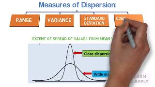
Just like that I want to give an idea about the normal distribution, but we will go in detail later. The next way to measure the dispersion is coefficient of variation. The ratio of standard deviation to the mean, express as a percentage.

So coefficient of variation is your sigma by mu, it is the measurement of relative dispersion. Already there is a standard deviation is there. What is the purpose of this coefficient of variations that will see the next slide?

Look at this, you see, stock A, stock B or stock 1,stock 2 the mu1 is 29, sigma1 is 4. 6. Another 1 mu 2 equal to 84, sigma 2 is 10, supposed to choose which is better.

If you compare only the mean, 29 verses 84, the second stock is better. Suppose if you compare the standard deviation, 4. 6 and 10.

The lower the standard deviation better it is. So the stock 1 is better. Now there is a contradiction, with respect to mean option B is better with represent standard deviation option A is better.

Now there is a contradiction to need to have the trade off. In this situation we have to go for this coefficient of variation, coefficient of variation is your Sigma 1 greater than mu. For example, for this case it is a 4.

6 divided by 29 multiply by 100 is 15. 86, for second case it is sigma 2 divided by mu 2, 10 divided by 84 multiply by 100 is 11. 90.

Lower the coefficient of variation, but have the option is. So, if the variance is smaller, to be able to choose that group, or that stock. Now we will see how to find the variance and standard deviation of the grouped data.

Already we have seen the standard deviation of the raw data also named as ungrouped data. We are seeing the standard deviation for population, standard deviation for sample. Similarly, we will find the variance for a grouped data.

So the formula is sigma f into M- mu whole square divided by N. Here, f is the frequency, M is the midpoint of that interval, mu is the mean of the interval, N is some of all frequencies. For the sample variants, look at the formula here it is also n-1, so sigma f of M -X bar squared divided by n-1.

So we will see this example now look at this, there with the grouped data is given; but the problem is given in the form of table. So, see these are the interval. These are frequencies.

So 20 to 30, there are six values are there. Between 30 and 40 there are 18 values is there, 40 and 50,11 is there 50 and 60, 11 is there. 60 and 70, 3 is there, and so on.

So first 1 we are to find out the midpoint of the interval between 20 and 30, the midpoint is 25, 35, Next interval 45, 55, 65, 75. Now, you multiply this f and the midpoint of the interval. So, 150,630, and so on.

We need this sigma f M then you can find M- mu, M is 25- 43- 18, 35- 43-8 and so on. Then you square it, then the squared value you multiply by f, you are getting this f into M- mu whole square . When you add it, that is going to be 7200, N is sigma of f.

There is nothing but 50. So 144 is the population variants of this grouped data. If you want to know the standard deviation of this group of data, just to take the square root of the variance, that is 12.

The next measure is shape of the, we can say a set of data. That is shape or distribution, what distribution follows. We can see the skewness, kurtosis, box and whisker plots there are the three method.

So we will see what is a skewness, skewness is the absence of symmetry. As I told you it may be this is left skewed data. This is a right skewed data.

This is symmetric data. So this absence of symmetry, this and this can be done with helps skewness. So the other one the application of skewness is to find out what is the nature of this shape, whether it is skewed or symmetric.

Next one is a kurtosis; it is the peakedness of a distribution. There are three layers, there are Leptokurtic, Mesokurtic, Platykurtic. Leptokurtic means high and thin, Mesokurtic is little flat in this way and Platykurtic very very very very flat this way flat and spread out.

Then we can see, box and whisker plots. It is a graphical display of distribution. It reveals skewness.

The application of boxer whisker plot is to check whether the data, follow a symmetry or what is the nature of the skewness of the distribution. See the skewness left one which is an orange color it is the negatively skewed. As I told you the previous lecture skewness is how it is named is looking at the tail.

the tail is on the left hand side so it is a left skewed or negatively skewed. Come to the blue one, the extreme right. It is this tail is on the right hand side.

So it is a right skewed or positively skewed one, the middle one there is no skewness, so it is symmetric. The skewness of a distribution is measured by comparing the relative position of the mean, median, and mode. If the distribution is symmetrical, we can say mean equal to median equal to mode.

The distribution is skewed right, the median lies between mode and mean, and the mode is less than mean. The distribution skewed right means this way. So this will be our mean, this will be our median, this will be mode.

Look at this, Median lies between mode and mean. The mode is less than the mean because mode is less than the mean. The same thing the distribution is skewed left.

This is the case. So the mean position of mean will be here. Median position of the mode, the median is lies between mode and mean.

And the mode is greater than mean. As I told you, whenever, if you want to know the central tendency of your distribution you to check the nature of the distribution. If it is skewed right or left, you should go for median, because the median always middle of the distribution irrespective of your skewness.

The same thing, what are explained the previous one. Mean, see negatively skewed the position of mean is here, median, mode. Positively skewed to the position of means here, median is here, mode is here.

There is no skewness in middle one. How to find coefficient of Skewness? The summary measure for Skewness can be measured as S equal to 3 to mu – median divided by sigma.

If S is negative, it is negatively skewed. If S equal to 0. It is symmetric.

If S is greater than 0, the distribution is positively skewed. You will see an example. Mu1 is 23, median1 is 26, sigma1 is 12.

3, and you apply this formula, 3 into 23- 26 divided by 12. 3 we are getting negative, so it is a negatively skewed. Go to the middle one mu2 equal to 26, median2 equal to 26, so 26, 26 it is equal to 0.

So S2 equal to 0. For this distribution the skewness is 0 or it is symmetric. The right one Mu3 equal to 29, median is 26, Sigma3 is 12.

3, and you substitute here we are getting positive value for S3. So the skewness is positive. The kurtosis, as I told you, it is a peakedness of a distribution, when they say Leptokurtic, leptokurtic, this one.

So it is high and thin, if that means highly homogeneous distribution, the things are very close. This is second one is the Mesokurtic, it is normal shape. The last one is Platykurtic, flat and spread out.

The next we will go to box and whisker plot. There are five positions in the box and whisker plot. One is median Q2, first quartile Q1, third quarter Q3.

The next word is the minimum value in the data set, maximum value in the data set. We will see this one here, this one. So, this point is would minimum value in this box is a Q1 is the quartile one, quartile two, quartile three maximum, why its called box and whisker plot.

The whisker is look like a whisker of a cat. So it is a box and whisker plot. You see how the skewness can be measured or identified with the help of box and whisker plot.

So by looking at the position of this middle this line, we can identify the distribution. What is that, if it is on the right side of this box it is left skewed data. If it is a left side it is the right skewed data.

If it is exactly on the middle, it is symmetric which follow normal distribution. So far, we have given some kind of theories about this various central tendencies and dispersion. Now, I'm going to switch over to Python.

So whatever we have done. The theory portion whatever we are taught here, so I am going to use Python. I am going to explain how to use Python to get central tendencies, skewness, box and whisker plot and various dispersion techniques with the help of Python.

So we will go to the Python mode. (Video Starts: 16:26) Okay, now we will come to the Python environment, the first, as I told you we are to import pandas as pd. We can do this pd is it is for only our convenient fantasies and library.

Then they are to the import Numpy numerical Python, as the np. Okay, so the first one is to import the required libraries. The second one is going to import the data set.

So the data set, already I know the part of the data set is the otherwise the name of the data set is IBM underscore 313 marks. xlsx. So, I am going to save the object called Table.

Table equal to pd. , this is the command. This read_excel is the command for the reading the Excel file.

The path is this, ‘IBM-313’ otherwise; simply you can type it there. Now print table, let us see what is the data. See, look at this, serial number is there, MTE that is a midterm examination marks, mini project, total, end term examination marks and total marks.

Okay, this total is out of 100, this total is out of 50. You see it is starting from 0,1,2,3. Okay, now I want to find out the mean of the total that is in the end term examinations.

So, x = table, the object either be a square bracket. There you have to write the column name. So that means I am going to take only the column name, total, and I go to store that value into the variable x.

Now the x is nothing but by the last column, if you want to mean of that one. So, np. mean.

Otherwise, if you want to know np. If you press tab you will get various options to that np. tab.

See here, there are so many options there in that have there are maximum, minimum, the mean, median, you need not remember also you can check it one by one. So now we will go to the np. mean.

Then, np. mean, then we will call that variable x executed, shift enter. So we are getting this value 46.

90 is the average marks. There is a lot of the median. So np.

median, median is 45. We will go for mode, the mode. You have to import scipy, from scipy import stats.

Stat is another library function. So start stats. mode called the variable x.

We will see what is the mode? Mode is the number of frequencies. Suppose, there are five students see got the same marks 30 bars, the mode will be 30.

Okay. So, okay, we will come back to later. So, next we will go to percentile.

In percentile suppose I have taken the array, that we are introducing another one np. array, a equal to np. array just we have taken an array 1, 2, 3, 4, 5.

Suppose, go to say p equal to np. percentile of that array a, 50. What do you want to know?

I want to know 50th percentile, 50th percentile means what value in this array will be the 50th percentile, and execute this print P. So, 3 is the 50th personality but the median. This number is very small number one for illustration purpose.

So you can have a large number then you can run it. Then now, we will go to another command in Python is for loop. For loop is suppose I have taken a variable k saved three variables, one is Ram, Seeing the characters in the code 65, 2.

5. Suppose if I print k, what will happen. You see that it is printing Ram, 65, 2.

5. But there is a requirement that I have to print one by one. First I have to print Ram, and then I have to print 65, and then print 2.

5. Now here at a time I am getting all the answer but I want to print one by one. So for that purpose, see that for i in k.

This is the syntax, there should be a colon, that is one print i. So what will happen first in k this is array. So first, for i in k will take the value Ram, second i will take the value of 65.

Third, i will take the value of 2. 5. Now if we execute this print i, see that one by one.

So this is the one by one, I am getting this output. So this is the example of for loop. So for i in k.

the k is in which variable. So the i value will change. if you want to print i.

So the first it print Ram and then 65 and 2. 5, because why I am showing that we are going to use this for loop incoming examples. So I want to give an idea about how to use for loop in Python.

Now we will go to the range. So, far i in range. Is it that 10, 20, 2 this is the rage function.

The rage first one is the starting value. The second one is the ending value, the 2 is increment; print i. if we print that you see that, now what is happening.

10, 12, 14, 16, 18 incremented by 2, ending with excluding 20. 1, 2,3,4,5 increment is by 2. Now suppose in the print, I want to print, now it is printed one by one.

But I want to print in i with the comma, so 10, 12, 14 that purpose the same comment, i use end equal to it should be separated by a comma in colon. So if I run this. What is happening see 10, 12,14,16,18 so this one end equal to in colon comma.

That is what how it is giving the output in horizontal way. Now we will go to the next option functions in Python. Suppose the functions are very useful applications in Python many time.

There are some built in function is there. For example; print is the built in function, maximum is the built in function, and minimum is built in function. You can create your own functions, and then you can call that function wherever it is required.

Suppose def,that is the syntax def greet open parenthesis, end with the colon, print Hi, print good evening. So, this is the way of defining your function. Okay, then.

After defining the function, you have to call that function, suppose I call the greet. I will execute this word what will happening? So, this function is getting executed.

So again Hi, and good evening. So another example or function suppose I want to add two numbers, so def the function name is add in parenthesis, p,q. It can be anything colon, the colon is important.

Otherwise, it will show syntax error. So c equal to p+q, so print c. suppose this is my function, suppose this is, I want to call this function, add 6,4 what answer I am getting.

Suppose other number suppose, add 10,4. So I am getting 14. We have seen how to create a function now finding the minimum, maximum value in the data set.

Suppose I created a new array. Data equal to 1, 3,4,463,2,3,6, just i take randomly. Suppose I want to see the minimum value in this array and maximum value in this array.

So what is happening. So minimum value is 1, the maximum value is 463. So for that the comment is min and max.

Now, this minimum and maximum value, I can create own function. Then I can call that function. Because every time I need not type minimum, min data, max data.

Because already that was built in function, we can create our own function. So the same data I have taken, 1, 3, 4, and 463. I am defining function min underscore; underscore MAX data, so min underscore value equal to minimum data, maximum underscore value equal to maximum data.

Now returns because I want to get the output. This is indentation is more important. Suppose, there is, minimum_value should be the same, same indentation, generally we can give Tab.

Tab means we can save for space work. So return underscore, minimum_value, maximum_value will run it let us see what is happening. So I am getting this because I called this function again how?

Min_and_max( data). Because my function name is Min_and_max. So 1, 463.

So this functions application is very much useful in Python because when you are making a large program, every time some routine aspects you need not do it, yourself every time. So you can call that function whenever it is required. It will save a lot of your time and energy.

So now, suppose I want to know the range of the data range is nothing but maximum value and minimum value. For that, I go to define a function def, that function name is rangef. That is the rangef.

rangef I given you can give any name for the data. So, I am finding minimum value equal to min of data, maximum value equal to maximum data return maximum_value minus minimum_value. So if i call that function rangef data, what will happenning I getting 462,nothing but 463-1.

Now we will go to quartile. Quartile, we have seen already. It is a Q1, Q2, Q3.

Q1is the 25th persentile, there is an inbuilt function in NumPy. So when you say I am creating an array, a equal to np. array, array1, 2,3,4,5.

So Q1 equal np. percentile. This np.

percentile will give you the percentile. Suppose if you want to know 25th percentile I can get what value in this array is the 25th percentile. So if I execute this.

So, that means, the value in two is 25th percentile. So the same thing np. percentile(a,50), if I put.

I am going to call it Q2. So 3 is, otherwise median you see look at this because it is odd number, the middle value three obviously it is the 50th percentile. I will go for third one, Q3 = 4.

That is our 75th percentile. Next, spredness is measured in terms of Inter quartile range. As we know already, Q3-Q1, so that is nothing but IQ.

So if we see IQ, there is nothing but Q3-Q1, 2 is inter quartile range. Now, we will go for how to find out the variance. Suppose, there are two way two variants one variances for fine variants of mean, another one is the variance of the population.

Even you put np. NumPy, var is for the population variance x. So what is the x, x is the total.

So that column, the total column we have saved in the name of object called x or variable called x. So we will see variance is 262. 781.

Suppose, there is a another function will be import to library statistics. So statistics. pstdev, that is population standard deviation x.

so I can get the population standard deviation, that is 16. 2105. It is the standard deviation.

So if you want to know the standard deviation of the sample. So, statistics. stdev.

So only thing is, if you want to know the population standard deviation, you should write p there, np. std otherwise by default, in statistics library, you are getting only the sample standard deviation. This is standard deviation for the population.

This is standard deviation for the sample. Next round for the skewness for that you are to import from scipy there is a library called dot stats import skew, skewness of x. So skewness is positive value so it is the right skewed data.

Next we will go to Box and whisker plot, because for drawing plot you have to use Matplotlib. Import pyplot as plt. So plt.

boxplot, there is an inbuild function as x comma symbol is star (*) plt. show execute this. So we are getting box and whisker plot.

You see that box and whisker plot rather than some star symbol that implies that that data is are outlier. Outlier means which goes beyond maximum value beyond minimum value. The position of this middle line will help you to identify the nature of the distribution.

If it is in left side, it is right skewed data. See, look at this, because it should positively skewed data and now it is little left side. So the data is, data is right skewed data.

So with that we are stopping the central tendency. So what we have seen so far we have seen various central tendencies and different way of measuring the dispersions, (Video Ends: 31:40) Whatever you will learn theory part that we run in Python, we got the answer. There are so many sources are available in internet to know the different course, different videos find out you can also refer that for this class.

Thank you.