An introduction to Policy Gradient methods - Deep Reinforcement Learning
213.93k visualizzazioni3743 ParoleCopia testoCondividi

Arxiv Insights
In this episode I introduce Policy Gradient methods for Deep Reinforcement Learning.
After a genera...
Trascrizione del video:
hi everybody welcome back to archive insights so lately we've seen a lot of new emerging algorithms in deep reinforcement learning and in this episode I want to dive into one specific algorithm called proximal policy optimization that was designed at opening eye and has proven successful on a wide variety of tasks going all the way from robotic control to Atari and even playing complicated video games like dota 2 now in this episode I'm gonna dive into some pretty technical terrain so I think it's good if you're a little bit prepared I've made a few previous videos
with an introduction to reinforcement learning and the problem of the sparse reward setting so I think if you're kind of new to the field of reinforcement learning I would suggest to watch those videos first and then come back to this video as we're going to dive pretty deep into the rabbit hole and being well-prepared definitely as a must for this video but if you think you're ready for it grab a cup of coffee and get ready to dive in deep because this episode is on proximal policy optimization my name is Xander and welcome to our
kevinsites [Laughter] [Music] all right so let's start by sketching some surroundings first so if we're doing supervised learning on a data set like image net for example then we can have a static training data set we can run a circus in gradient descent optimizer in that data and we can be pretty sure that our model will converge to a pretty decent local optimum the road to success in reinforcement learning however isn't that simple so one of the problems that reinforcement learning suffers from is that the training data that is generated is itself dependent on the
current policy because our agent is generating its own training data by interacting with the environment rather than relying on a static data set as is the case in supervised do and so this means that the data distributions of our observations and rewards are constantly changing as our agent learns which is a major cause of instability in the whole training process an apart from having this problem with varying training data distributions reinforcement learning also suffers from a very high sensitivity to hyper parameter tuning and things like initialization for example and in some cases it's kind of
intuitive to understand why this happens because imagine that your learning rate is too large well then you could have a policy update that pushes your policy network into a region of the parameter space where it's going to collect the next batch of data under a very poor policy causing it to never recover again and so to address many of these annoying problems in reinforcement learning the team and opening I designed a new reinforcement learning algorithm that's called proximal policy optimization or PPO and the core purpose behind PPO was to strike a balance between ease of
implementation sample efficiency and ease of tuning now the first thing to realize about PPO is that it is what we call a policy gradient method and this means that unlike popular key learning approaches like dqn for example that can learn from stored offline data proximal policy optimization learns online and this means that it doesn't use a replay buffer to store past experiences but instead it learns directly from whatever its agent encounters in the environment and once a batch of experience has been used to do a gradient update the experience is then discarded and the policy
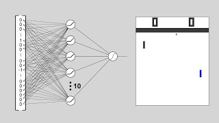
moves on and this also means that policy gradient methods are typically less sample efficient than queue learning methods because they only use the collected experience once for doing an update and our general policy optimization methods usually start by defining the policy gradient laws as the expectation over the log of the policy actions times an estimate of the advantage function okay so what is that only well the first term pi theta is our policy it's a neural network that takes the observed States from the environment as an input and suggests actions to take as an output
and the second term is the advantage function a which basically tries to estimate what the relative value is of the selected action in the current state so let's take apart what that means so in order to compute the advantage we need two things we need to discounted sum of rewards and we need a baseline estimate so the first part is the discounted sum of rewards or the return and this is basically a weighted sum of all the rewards the agent Gaad during each time step in the current episode and then the discount factor gamma which
is usually somewhere between 0.9 and 0.99 accounts for the fact that your agent cares more about reward that is going to get very quickly versus the same reward it would get a hundred times that for now and this is exactly the same idea as interest in the financial world in the sense that getting money tomorrow is usually more valuable than getting the same amount of money say a year from now and so notice that the advantage is calculated after the episode sequence was collected from the environment so in other words we know all the rewards
so there is no guessing involved in computing the discount or return because we actually know what happened okay so that was the first part of the advantage function the discounted sum of rewards and then the second part of the advantage function is the baseline or the value function and basically what the value function tries to do is give an estimate of the discounted sum of rewards from this point onward so basically it's trying to guess what the final return is going to be in this episode starting from the current state and during training this neural
net that's representing the value function is going to be frequently updated using the experience that our agent collects in the environment because this is basically a supervised learning problem you're taking States as an input and your neural net is trying to predict what the discounted sum of rewards is going to be from this state onwards so basic supervised learning and notice that because this value estimate is the output of a neural net this is gonna be a noisy estimate there's gonna be some variance because our network is not going to always predict the exact value
of that states so basically we're going to end up with a noisy estimate of the value function okay so now we have the two terms that we need we have the discounted sum of rewards that we computed from our episode rollout and we have an expectation an estimate of that value given the state that we're in and if we then subtract the baseline estimate from the actual return we got we get what we call the advantage estimate and so basically the advantage estimate is answering the question how much better was the action that I took
based on the expectation of what would normally happen in the state that I was in so basically was the action that our agent took was it better than expected or was it worse and so then by multiplying the log probabilities of your policy actions with this advantage function we get the final optimization objective that is used in policy grading and if you think about what this objective function is doing it's intuitively satisfying because if the advantage estimate was positive meaning that the actions that the agent took in the sample trajectory resulted in better than average
return what we'll do is we'll increase the probability of selecting them again in the future when we encounter in the same state and if on the other hand the advantage function was negative then we'll reduce the likelihood of the selected actions which makes total sense right and as I've already mentioned one of the problems is that if you simply keep running gradient descent on one batch of collected experience what will happen is that you'll update the parameters in your network so far outside of the range where this data was collected that for example the advantage
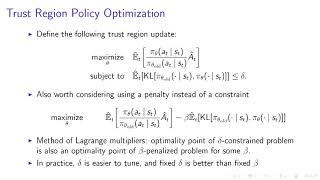
function which is you know in principle a noisy estimate of the real advantage is going to be completely wrong and so in a sense you're just going to destroy your policy if you keep running gradient descent on a single batch of collected experience and I'll to solve this issue one successful approach is to make sure that if you're updating the policy you're never going to move too far away from the old policy now this idea was widely introduced in a paper called trust region policy optimization or T RPO which is actually the whole basis on
which PPO was built and so here is the objective function that was used in T RPO and if you compare this we the previous objective function for vanilla policy gradients what you can see is that the only thing that changed in this formula is that the log operator is replaced with the division by PI theta old now the slide here shows that optimizing this TR Pio objective is in fact identical to vanilla policy gradients I'm not going to go into the derivation details here but if you want you can pause the video or check out
lecture 5 of the deep RL bootcamp which will take you deep down the rabbit hole link in the description now to make sure that the updated policy doesn't move too far away from the current policy TRP row adds a KL constraint to the optimization objective and what this Cal constrained effectively does is it's just going to make sure that the new updated policy doesn't move too far away from the old policy so in a sense we just want to stick close to the region where we know everything works fine the problem is that this Cal
constraint adds additional overhead to our optimization process and can sometimes lead to very undesirable training behavior so wouldn't it be nice if we can somehow include this extra constraint directly into our optimization objective well as you might have guessed that is exactly what PPO does ok so now that we have a little bit of surroundings let's dive into the crux of the algorithm the central optimization objective behind PPO hold on to your heads it's about to get a little technical the first let's define a variable R theta which is just a probability ratio between the
new updated policy outputs and the outputs of the previous old version of the policy Network so given a sequence of sampled actions and States this R theta value will be larger than 1 if the action is more likely now than it was in the old version of the policy and it will be somewhere between 0 and 1 if the action is less likely now than it was before the last gradient step and then if we multiply this ratio R theta with the advantage function we get the normal TRP or objective in a more readable form
and with this notation we can finally write down the central objective function that is used in PP oh here it is look surprisingly simple right well first of all you can see that the objective function that PPO optimizes is an expectation operator so this means that we're going to compute this over batches of trajectories and this expectation operator is taken over the minimum of two terms the first of these terms is R theta times the advantage estimate so this is the default objective for normal policy gradients which pushes the policy towards actions that yield a
high positive advantage over the baseline now the second term is very similar to the first one except that it contains a truncated version of this R theta ratio by applying a clipping operation between 1 minus epsilon and 1 plus epsilon where epsilon is usually something like 0.2 and then lastly the min operator is applied to the two terms to get the final result and while this function looks rather simple at first sight fully appreciating all the subtleties at work here takes a little bit more effort so bear with me here I promise we're almost there
firstly it's important to note that the advantage estimate can be both positive and negative and this changes the effect of the main operator here is a plot of the objective function for both positive and negative values of the advantage estimate so on the left half of the diagram where the advantage function is positive or all the cases where the selected action had a better-than-expected effect on the outcome and on the right half of the diagram we can find situations where the action had an estimated negative effect on the outcome now on the left side notice
how the loss function flattens out when R gets too high and this happens when the action is a lot more likely under the current policy than it was under the old policy and in this case we don't want to overdo the action update too much and so the objective function gets clipped here to limit the effect of the gradient update and then on the right side where the action had an estimated negative value the objective flattens when R goes near zero and this corresponds to actions that are much less likely now than in the old
policy and it will have the same effect of not overdoing a similar update which might otherwise reduce these action probabilities to zero remember the advantage function is noisy so we don't want to destroy a policy based on a single estimate and finally what about the very right hand side well the objective function only ends up in this region when the last gradient step made the selected action a lot more probable so are as big while also making our policy worse since the advantage is negative here and if that's the case then we would really want
to undo the last gradient step and it just so happens that the objective function in PPO allows us to do this the function is negative here so the gradient will tell us to walk the other direction and make the action less probable by an amount proportional to how much we screwed it up in the first place and also notice that this is the only region where the unclipped part of the objective function has a lower value than the clipped version and those gets returned by the minimization operator pretty clever right and if you're wondering how
on earth the authors from the PPO paper managed to design this specific reward function well it's quite likely that they had an intuitive idea of what they wanted the objective function to do so they probably sketched a bunch of diagrams that satisfied the behavior that we just discussed and then came up with the exact objective function to make it all work out and don't worry if you didn't fully get all the little details involved basically the PPO objectives does the same as a TRP all objective and that it forces the policy updates to be conservative
if they move very far away from the current policy the only difference is that PPO does this with a very simple objective function that doesn't require to calculate all these additional constraints or KL divergences and in fact it turns out that the simple PPO objective function often outperforms the more complicated variant that we have in T RPO simplicity often wins all right nice now that we've seen the central objective function behind PPO let's take a look at the entire algorithm end to it so as mentioned before there are two alternating threads in PPO in the
first one the current policy is interacting with the environment generating episode sequences for which we immediately calculate the advantage function using our fitted baseline estimate for the state values and then every so many episodes a second thread is going to collect all that experience and run gradient descent on the policy network using the clips PPO object and as was done in training the opening i-5 system these two threats can actually be decoupled from each other by using thousands of remote workers that interact with the environment using a recent copy of the policy Network and a
GPU cluster that runs gradient descent on the network weights using the collected experience from those workers note that in this case each worker has to refresh its local copy of the policy network pretty often to make sure that it's always running with the latest version of the policy network to keep everything nicely balanced now importantly the final loss function that is used to Train an agent is the sum of this clips PPO objective that we just saw plus two additional terms the first additional term of the loss function is basically in charge of updating the
baseline network so this is the part of the network graph that is in charge of estimating how good it is to be in this state or more specifically what is the average amount of this counted reward that I expect to get from this point onwards so even though the value and policy outputs form two separate heads of the same network because they are part of the same computation graph you can actually combine everything in a single loss function and the auto differentiation library will just figure out where to send all the gradients and the reason
that these two lost terms are actually part of the same objective function is that the value estimation network shares a large portion of its parameter space with the policy Network and the intuition is that whether you're trying to you know estimate the value of the current state or you simply want to take the best current action well you're likely going to need very similar feature extraction pipelines from the current state observation so these parts of the network are simply shared and then finally the last term in the objective function is called the entropy term and
this term is in charge of making sure that our agent does enough exploration during training so in contrast to discrete action policies that output the action choice probabilities the people your policy head outputs the parameters of a Gaussian distribution for each available action type and when running the agent and training mode the policy will then sample from these distributions to get a continuous output value for each action head now if you want to fully understand why the entropy term encourages exploration I really recommend to check out ugly Angelo's video on the ideas behind entropy and
KL divergence in machine learning the link is in the description but basically the entropy of a stochastic variable which is driven by an underlying probability distribution is the average amount of bits that is needed to represent its outcome it is a measure of how unpredictable an outcome of this variable really is and so maximizing its entropy will force it to have a wide spread over all the possible options resulting in the most unpredictable outcome and so this gives some intuition as to why adding an entropy term will push the policy to behave a little bit
more randomly until the other parts of the objective start dominating and as always we have a couple of hyper parameters C 1 and C 2 that way the contributions of these different parts in the loss function now for people that want to take a deeper look at PEO in terms of Python code I really recommend to check out this implementation in PI towards from our L adventure trust me even though you've never worked with PI torch this implementation is as clean as it gets and if you're looking for a more production proof implementation I would
recommend to check out opening eye baselines which has a full implemented tensorflow version that runs on different environments like Atari Mojo Co and others both links are in the description all right so that's it congratulations if you've made it this far we've covered all you need to know about proximal policy optimization now in the paper you can find a bunch of graphs that compare PPO to other benchmarks in deep RL so don't hesitate to have a look the link is in the description the important thing to remember though is that PPO wasn't specifically designed for
sample efficiency but rather to address the really complicated code that was needed for a lot of other algorithms and also you know making it relatively easy to tune in terms of high performers and because PPO achieves both of those objectives while also yielding close to or above state-of-the-art performance on a wide range of tasks it has become one of the benchmarks in deep reinforcement learning so in summary PPO is a state of the art policy gradient method the algorithm has the stability and reliability of T RPO while much simpler to implement requiring only a few
tweaks to vanilla policy gradient methods and it can be used for a wide range of reinforcement learning tasks great or before I end this video I would really like to thank all the people that support this channel on patreon I mean even if it's only $1 a month those contributions really mean a lot to me they are a big motivation because they show that the people out there really care for the content that I'm making and it's a really good motivation to keep going so thanks a lot all my great amazing patreon supporters if wha
that was it for this episode thank you very much for watching I hope you learned something about proximal policy optimization don't forget to Like subscribe and share and I'd love to see you again in the next episode of archived insights [Music]
Video correlati
16:27
An introduction to Reinforcement Learning
Arxiv Insights
671,851 views
1:02:47
Proximal Policy Optimization (PPO) is Easy...
Machine Learning with Phil
70,923 views
59:36
Policy Gradient Theorem Explained - Reinfo...
Elliot Waite
67,034 views

16:01
Reinforcement Learning with sparse rewards
Arxiv Insights
119,794 views
29:05
Policy Gradient Methods | Reinforcement Le...
Mutual Information
40,948 views
17:50
Proximal Policy Optimization Explained
Edan Meyer
56,143 views

13:26
Proximal Policy Optimization | ChatGPT use...
CodeEmporium
23,510 views
1:07:30
MIT 6.S091: Introduction to Deep Reinforce...
Lex Fridman
309,092 views
41:01
Deep RL Bootcamp Lecture 5: Natural Polic...
AI Prism
53,715 views

21:37
Reinforcement Learning Series: Overview of...
Steve Brunton
111,643 views
1:19:37
Paper: DeepSeek-R1: Incentivizing Reasonin...
Umar Jamil
29,742 views

1:09:00
DeepSeekMath: Pushing the Limits of Mathem...
Yannic Kilcher
81,485 views
36:26
A friendly introduction to deep reinforcem...
Serrano.Academy
110,385 views
21:24
PPO Implementation from Scratch | Reinforc...
Papers in 100 Lines of Code
673 views
56:31
Deep RL Bootcamp Lecture 1: Motivation + ...
AI Prism
96,353 views
41:22
L3 Policy Gradients and Advantage Estimati...
Pieter Abbeel
31,811 views
38:24
Proximal Policy Optimization (PPO) - How t...
Serrano.Academy
36,023 views

27:22
AI Is Making You An Illiterate Programmer
ThePrimeTime
147,149 views
9:54
Why humans learn so much faster than AI
Arxiv Insights
49,718 views
8:25
Reinforcement Learning from scratch
Graphics in 5 Minutes
106,984 views