Bode Plots by Hand: Complex Poles or Zeros
439.82k views2009 WordsCopy TextShare
Brian Douglas
Get the map of control theory: https://www.redbubble.com/shop/ap/55089837
Download eBook on the fund...
Video Transcript:
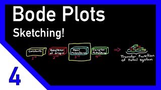
welcome back to control system lectures this video is a continuation of the series that we've been doing on approximating Bodi plots by hand we're going to wrap up this topic for now with this fourth and final video at the end of this lecture you should have all of the necessary tools you need to approximate the frequency response of any transfer function we have already covered transfer functions that are constants which is a transfer function that has no poles or zeros and we've also covered transfer functions that have a real Pole or zero at the origin
and the last video covered transfer functions that have real poles or zeros that aren't at the origin so far all of our discussions have been about poles and zeros that lie somewhere along this real line none have ventured out into the imaginary realm until now in this lecture I'll explain how to draw an approximation of the bod plot by hand for a function with a pair of complex poles or zeros and by pair I mean two poles or zeros that are symetric about the real line in other words the imaginary component have equal magnitude but
opposite signs so why a pair and not a single complex polar zero well I'm glad you asked let me explain it this way a transfer function with a single complex pole might look something like this 1 / s+ J and this function has a single pole at s = minus J and mathematically this is a perfectly legitimate transfer function however we need to remember that transfer functions aren't just mathematically abstract functions they represent real physical objects and so now the question is what physical first order object could this complex transfer function represent I'll give you
two quick examples A first order mechanical system could be a massless spring damper system with spring constant K and damping coefficient B and the transfer function could be written like this and now in order for the this transfer function to have imaginary Roots either the damping coefficient or the spring constant has to have an imaginary value which for a physical system doesn't make sense if we take an electrical example we could have a circuit that has an inductor and resistor in series where the inductor has inductance L and the resistor has resistance R and the
transfer function for this first order system would look similar to the mechanical system it would be 1 / LS S Plus R and now we're left with the same problem what does it mean to have an inductance or resistance that has an imaginary value now something to think about here is what would a physical system look like that had an imaginary value for one of its properties so in both of these cases the coefficients of the transfer function polinomial all have real numbers and that's because they represent real physical values like spring constants and inductance
and resistance other physical properties are things like torque or pressure or flux or current or volume and all of these have real values even if a transfer function has pols that have real coefficients it's still possible to have imaginary Roots but in order to do so we must have a second order system or higher this can be seen from this generic second order equation you can solve for the roots of this equation using the quadratic equation which is minus B plus orus < TK b^ 2 - 4 a c all 2 a in order to
have complex Roots the value inside the square root must be negative and you can see that this is true when 4 a c is greater than b ^2 and if we took the ratio of these two you could say that when the square root of b^2 / 4 a is less than one then we'll have complex Roots this is called the damping ratio and it's assigned to the Greek letter Zeta this ratio is important in control systems since it marks the boundary between complex Roots I.E oscillatory motion and real Roots which is exponential motion so
let's continue on with our idea let me rewrite the quadratic equation in this form you can see that the right side of the equation could be either real or imaginary based on the damping ratio Zeta but the left side of the equation equ is always a real value so now you can see that if we have complex Roots the real portion will be the same for both roots and the imaginary portion will have the same magnitude but opposite signs of each other and these are called complex conjugates we can show this graphically on a real
imaginary axis like this the two complex Roots will always be mere images of each other across the real line and this is why for real physical systems complex Roots will always come in pairs and always be complex conjugates of each other now that we have that understanding let's get to the math and learn how to draw the frequency response of a system whose transfer function have two poles that are complex conjugates the form of this type of transfer function could be written like this omega^2 / s^ 2 + 2 zaeta Omega s+ omega^2 but like
we did in previous videos we want to manipulate the form into this structure by dividing both the top and bottom by Omega KN squ at this point solving for the frequency response is no different than for simpler transfer functions first you have to substitute s equals J Omega and then solve for the real part and the imaginary part of the equation the only difference here though is that this equation is a bit more complicated than the previous ones we looked at so the algebra can get a bit unwieldy I assure you though I'm performing the
same mathematical steps that I did in previous videos I always recommend you trying this on your own though one to verify that my math is correct and two practicing it helps you to retain the knowledge the white bit at the end here is multiplying the top and bottom by the complex conjugate of the denominator in order to move the imaginary number J to the numerator and once you've multiplied those equations together and you separate out the real component and the imaginary component you should end up with two giant equations that look similar to these and
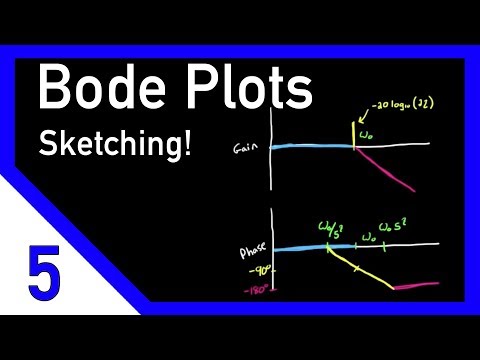
now if these haven't scared you off then we can use the real and imaginary components to estimate the magnitude and the phase across the entire frequency spectrum we'll start by drawing our empty Bodi diagrams one for gain and one for phase then we'll mark in the middle here somewhere where our break frequency Omega KN is and as you're used to by now we'll break our estimation up into three different cases the first where Omega is much smaller than than Omega KN in this case Omega over Omega KN goes to zero and the real part simplifies
just to one and for the imaginary component it can be approximated as zero since the numerator goes to zero when Omega is really small now the magnitude of H of J Omega is just 20 * the log base 10 of the square root of the real component squared plus the imaginary component squar which turns out to be 0 DB we can just draw this in on the gain plot up to the break frequency remember this is just an approximation not an exact plot for phase it's the argument of H of J Omega which is the
arc tangent of the imaginary part divided by the real part which is just 0 degrees up to the brake frequency the second case is when Omega is much greater than the brake frequency in this case Omega over Omega KN dominates the equation and the real component can be approximated as Omega over Omega KN to the -2 power and the imaginary component can be approximated as 2 Zeta Omega over Omega to the -1 power to find the magnitude note that the real component is much smaller than the imaginary component because it has a square rather than
a single power so as Omega gets larger and larger and larger the magnitude is going to follow the trend of the real component which is minus 40 DB per decade so we can draw that line in starting at the breake frequency as for phase I made a mistake here in my intermediate step but it's too difficult for me to go back and correct it at this stage so I'm just going to have to leave it for now but the phase at these higher frequencies does come out to be minus 180° so we can draw that
in starting at the breake frequency for the third case Omega equals The Brak frequency Omega KN now the ratio Omega over Omega KN equals 1 the real component is zero and for the imaginary component you're left with with - 2 Zeta / 2 zaa 2 or just -1 / 2 Zeta now for the game plot this is worth noting the magnitude at the breake frequency is equal to 1 / 2 Zeta written in decb in other words as your damping ratio decreases your magnitude at this breake frequency increases all the way up to Infinity when
Zeta goes to zero notice that for zeta's larger than 0.5 this magnitude is going to be less than zero for that reason for the approximation we generally only draw a peak when Zeta is less than 0.5 phase however is slightly more tricky at the break frequency the phase goes to minus 90 degrees which is halfway between however the slope of the line that connects the blue line to the pink line changes as a function of Zeta now you can either look up the shape of the graph in a chart based on your Zeta or you
can draw it directly by drawing a line starting at Omega KN / 5 to the Zeta power all the way up to Omega KN Time 5 to the Zeta power now these three line segments for the gain and phase plots are just approximations of what the frequency response looks like the thick red line is the exact frequency response of the system and you could draw this Closer by just smoothing out the lines however generally what you're trying to find is the low frequency high frequency and break frequency characteristics which you can just do with a
straight line approximation now I've spent this entire time talking about complex poles but just like we did before we can approximate the frequency response of complex zeros by noting that a zero is one divided by a pole and on a log log scale of a bod plot this is just the negative of a complex pole so you can just reflect the response about the horizontal axis to get the response of a zero and this wraps up the segment on approximating bod plots by hand I apologize for the messy and confusion at the end here but
I hope that you have enough information to at least attempt this on your own being able to approximate a bod plot goes beyond just being able to draw some lines on a graph you should be able to understand how adding a pole or a zero to a transfer function changes the frequency response characteristics of a system this skill is invaluable when designing something like a PID controller or adding a filter to a signal to remove unwanted noise and so while you may never actually draw a b plot by hand you will always benefit from knowing
how thanks for watching and don't forget to subscribe
Related Videos
10:56
CORRECTION: Bode Plots by Hand: Complex Po...
Brian Douglas
292,949 views
12:45
Control System Lectures - Bode Plots, Intr...
Brian Douglas
1,251,048 views

Jazz & Work☕Relaxed Mood with Soft Jazz In...
Jazz For Soul

Music for Work — Limitless Productivity Radio
Chill Music Lab

Cozy Winter Coffee Shop Ambience with Warm...
Relax Jazz Cafe

1:19:51
J.S. Bach: The Violin Concertos
Brilliant Classics
30,124,767 views
13:54
Gain and Phase Margins Explained!
Brian Douglas
661,890 views
13:38
Bode Plots by Hand: Real Poles or Zeros
Brian Douglas
367,758 views
18:04
Signals and Systems - Bode Plots
UConn HKN
158,376 views

Christmas Jazz ☕ Smooth Jazz Coffee Music ...
Sweet Morning Cafe

13:10
The Root Locus Method - Introduction
Brian Douglas
1,074,843 views

Music for Work — Deep Focus Mix for Progra...
Chill Music Lab

December Jazz: Sweet Jazz & Elegant Bossa ...
Cozy Jazz Music
13:53
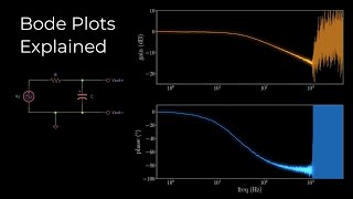
Bode Plots Explained
Curio Res
50,724 views

Productivity Music for Studying, Focus and...
Greenred Productions - Relaxing Music

Sweet Christmas Jazz ☕ Smooth Jazz Backgro...
Sweet Morning Cafe
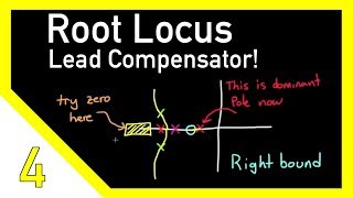
13:58
Designing a Lead Compensator with Root Locus
Brian Douglas
484,543 views
14:19
Designing a Lead Compensator with Bode Plot
Brian Douglas
367,971 views
![✅ DIAGRAMA DE BODE [Ceros y Polos Complejos Conjugados] #009](https://img.youtube.com/vi/IQpb9GLcv_A/mqdefault.jpg)
27:40
✅ DIAGRAMA DE BODE [Ceros y Polos Complejo...
Sergio A. Castaño Giraldo
28,439 views

Iron Man Workshop Radio — Work Music for C...
Chill Music Lab