NASA ARSET:  SAR for Flood Mapping Using Google Earth Engine, Part 1/3

hello and welcome to the first part of the advanced synthetic aperture radar webinar series for disaster and hydrological applications i'm dr erica podest and i'm a scientist in the earth science division at nasa's jet propulsion laboratory in pasadena california this series contains three trainings this one is focused on sar for flood mapping using google earth engine the second one on december 4th will focus on interferometric sar for landslide observations which will be taught by dr eric fielding from jpl and the third one on december 5th will focus on how to generate a digital elevation model

and will be taught by nicolas gruenfeld from konai the argentinian space agency each webinar will have a theoretical part and a demonstration today i'll begin with sar theory as related to flooding and i'll then go through a demo on how to generate a flood product with google earth engine this session builds on the previous flooding session using google earth engine each webinar will be done in both spanish and english on the same day there will be one homework associated with this webinar series and we will assign that homework on the last day it will be

in google form to obtain a certificate of completion you must have attended all parts of the series and submit the homework by the due date which is january 8 2020 in all of the demos we have step-by-step instructions for you to follow and we will go at a certain pace through the demos but we will make the recordings available within 24 hours so you can go at your own pace learning objectives i expect that by the end of today's webinar you'll be able to understand the information content and star images relevant to flooding this is

actually a review of what's been presented in the past it's important that you understand why the radar signal is sensitive to flooding for those of you that have seen this already consider it a refresher i'll also show you how to use google earth engine to generate a flood map using sentinel 1 images in the previous webinar i did a demo using google earth engine to generate flood maps from sentinel 1 sar images by applying a threshold this demo will focus on generating a flood map to a supervised classification approach you'll also learn how to integrate

socioeconomic data to your flood map in order to identify areas at risk i'll start out by defining what is meant by flooding from a radar perspective it refers to the presence of a water surface underneath a vegetation canopy regardless of whether it is forest or agriculture when i refer to an inundated forest it means that underneath the vegetation canopy there is standing water above the soil surface as shown in the figure on the top left in agricultural or herbaceous areas the leaves or stems of the plants visibly emerge above the water surface as shown in

the bottom center figure radar can also detect flooding when or where there is no standing vegetation and i will call this open water such as the figure on the top right the type of flooding discussed in this webinar can be caused by natural processes such as the seasonal flooding of wetland ecosystems or as a result of a natural hazard for example hurricanes or extreme precipitation events some floods can also be human driven such as flooded rice fields assessing and monitoring flood extent can help reduce uncertainties in the spatial and seasonal extent of methane sources and

sinks associated with wetland ecosystems or the cultivational crops that require standing water such as rice also flood maps can help monitor inundation extent and dynamics for disaster assessment and management this slide is a refresher of the radar backscattering mechanisms in general emphasizing with the red boxes the ones that are primarily relevant to flooded vegetation and open water in the far left there's specular scattering and that occurs when there is a smooth surface such as a calm open water surface and the signal scatters away from the satellite in this example the signal is coming from the

left and scattering away from the satellite towards the right and this results in open water appearing very dark in the image the next type of scattering is rough surface scattering which results when there's some level of roughness on the surface causing the signal to scatter in different directions but mostly away from the satellite an example of this type of scattering would be a water surface that has some level of roughness caused by either short floating vegetation wind or heavy rain such an area would appear dark but not as dark as an open water surface that

is completely smooth the rougher the surface the larger the signal scattered back to the satellite and the brighter that pixel will appear on the image the next signal interaction is volume scattering and that occurs when the signal is scattered multiple times in multiple directions within a volume or medium in the case of vegetation the signal can scatter from multiple components such as the branches stems leaves trunks or the soil and the final backscatter mechanism on the far right is called double bounce and this results when two smooth surfaces create a right angle that deflects the

incoming radar signal off both surfaces causing most of the energy to be returned to the sensor these areas appear very bright in the image and are commonly seen when there is flooded vegetation because of the interaction between the smooth water surface and vertical structure of the vegetation such as a trunk double bounce is also characteristic of urban areas here we have an example of the sar signal scattering over areas of inundated vegetation and open water this figure is an l-band hh polarized image from the japanese palsar sensor onboard the halo satellite over an area near

manaus brazil the very bright white areas are flooded vegetation and the dark areas are open water so that river that's running through the middle is dark because open water is a smooth surface and causes specular scattering all of the very bright white areas throughout the image are flooded vegetation because of double bounce and the striking part about this image is that in some areas you can't see specular scattering from the river because it's the river is either too small or it's covered by vegetation but you can still see its extent through flooded vegetation because the

signal is penetrating through the canopy and double balance is occurring this level of detail on flooded vegetation is truly a unique attribute of radar the satellite parameters that influence the sar signal response are wavelength polarization and incidence angle i'll start with wavelength generally the longer the wavelength the greater the capability of the sar signal to penetrate through the vegetation canopy all the way to the surface the table on the right lists commonly used bands in radar and their wavelength range sars operating at x-band are generally operating at a wavelength of around three centimeters at c-band

at a wavelength of around five centimeters and at l-band at a wavelength of around 24 centimeters as you can notice this range is quite wide there have been several studies that have concluded that l band is suited to detect inundation beneath a forest canopy and should be the preferred wavelength for this purpose however that capability of l-band and also other bands to penetrate some forested areas can be reduced or even non-existent depending on the gaps in the canopy or especially on the density of the vegetation as an example a couple years ago i was part

of a team conducting wetland studies in the peruvian amazon and we overflew uavsar that's a jpll band airborne sensor over our site of interest and at the same time that we were overflying uavsar there was someone on the ground collecting in-situ data this person was in water up to his knees however the radar data did not see any flooded vegetation because the vegetation was simply too dense and the signal did not penetrate all the way down through the canopy in comparison to l-band the ability of shorter wavelengths such as c-band or x-band to penetrate vegetation

the vegetation canopy is reduced although the penetration of c-band is limited in comparison to l-band studies have shown an increase in sea band backscatter for flooded vegetation during leaf on conditions and especially during leaf off conditions seaband is especially useful if the density of the vegetation is low and works particularly well in agricultural regions or in areas of low biomass expand sensors for example terra srx in general have even more limited penetration through dense vegetation and as a result of high in interference with leaves where backscatter is dominated by volume scattering however there have been

some studies that have shown the potential of x-band to identify flooded vegetation for sparse vegetation or leaf off conditions in this case the transmittivity of the signal through the canopy is increased due to gaps in the canopy or the very low biomass and the contribution of double bounds dominating the volume scattering some other studies have demonstrated the ability of x-band to map flooded vegetation in wetlands in flooded marshland and in olive groves so in summary l band is better suited for dense vegetation but shorter wavelengths might give you reasonable results especially if there are many

gaps in the vegetation so the shorter wavelengths are better suited for low density vegetation polarization refers to the plane of propagation of the electric field of the signal which can be har in the horizontal plane or in the vertical plane irrespective of wavelength radar signals can be transmitted and or received in different modes of polarization and there can be four combinations of both transmit and receive polarizations and these are horizontally transmitted horizontally received horizontally transmitted vertically received hv vertically transmitted vertically received that's vv and vertically transmitted horizontally received ph penetration depth is influenced by polarization

in force hh tends to penetrate deeper into the canopy because it tends to be less attenuated than vv so hh is a better polarization to detect flooded vegetation especially in areas where there's a high biomass and you have something like l-band there's a higher likelihood that hh will penetrate through the canopy and detect that standing water underneath the vegetation canopy hv is more sensitive to volume scattering and is a good indicator of vegetation cover in general here we have an example of multi-polarization images from elos palsar over a part of the paccaya sumerian natural reserve

in peru which is a vast wetland ecosystem these are l-band images at hh hv and vvv polarizations the very bright areas are where double bounce dominates and this is where there's inundated vegetation the very dark areas are open water and you can clearly see the river through the middle of the image as well as some open water bodies north and south of the river note the difference in backscatter magnitude between the different polarizations if you focus on inundated vegetation or the very bright areas dominated by double bounds the hh polarization is the most useful one

for distinguishing flooded from non-flooded vegetation vv shows flooded vegetation to a lesser extent and even lesser by hp polarization so in general hh penetrates deeper into the vegetation canopy than vv and when striking the water surface is more strongly reflected in comparison to the vv polarization hv is more sensitive to volume scattering because of its depolarizing characteristics so this is an example of an rgb image containing different polarizations false color images are an ideal way to visualize the information content of different polarizations through color combinations because you can see the information content that's unique to

each polarization or combinations of polarizations here we have hh in the red channel hb in the green channel and vv in the blue channel the pink areas in the image are those where flooded vegetation is present here we have an example of the effect of incidence angle variation on the left is a sentinel 1 vv image and on the right is the incidence angle variation for this same image the radar is right looking and so note that as we move across the swath from near to far range the image becomes increasingly darker in tone around

a 3 to 5 db difference in backscatter so if you measure for example the same forest at different incidence angles then the measured backscatter will be different even if there has been no physical change in the forest every surface feature will have a backscatter value that is a function of incidence angle so you need to be careful when comparing backscatter of a feature when there is a large variation in incidence angle especially if your feature is at the end at the near range and the far range of the image incidence angle can especially affect the

appearance of smooth targets on the image such as open water smooth surfaces can appear brighter than rough surfaces at small incidence angles usually less than 20 to 25 degrees now let's discuss a source of confusion that might lead to errors when classifying open water and again this is a pulsar image it's near manaus brazil at three different polarizations hh hv and vvv and you can clearly see that the water is dark but north of the river there are areas that have either no vegetation or very low vegetation and so these areas can be confused with

open water because uh ultimately they they they're very smooth areas right there's very little scattering going on in these areas of low vegetation and so their their backscatter response is similar to open water especially if it's open water with some level of roughness because of the wind for example they can be easily confused and one way to clear this up is by using image ratios such as hh over hb so you also note in this example that hh and vv have a much higher sensitivity to roughness of on the water surface to to for example

wind and you can see that in hv open water is is very very dark it's much darker than an hh in bb so strictly to identify just open water hv is the better polarization [Music] another source of confusion that might lead to errors when classifying flooded vegetation are urban areas and here we have a pulsar image containing the city of manaus in brazil and its surroundings up in the northern part of the image and the image also shows flooded vegetation which has a very bright backscatter so you can clearly see all of the flooded vegetation

around the river and the city of manaus it's quite a large city it has a population of about 2.5 million people including its suburbs and the city appears very bright similar to flooded vegetation and the reason for this is because the dominating scattering mechanism is double bounce right angles form between smooth surfaces such as roads and vertical structures such as buildings causing this high return and one way to at least partly clear up this confusion between urban areas and flooded vegetation is through the use of texture measurements and textures they provide information about the statistics

of the pixels within a box and the size of the box is defined by the user some textures such as energy or entropy provide information about the homogeneity or inhomogeneity of the pixels within the box and in my experience such measures help separate urban areas from flooded areas because urban areas tend to be more homogeneous than flooded areas sar datasets have improved significantly in the last couple years and this list here shows the legacy current and future sar data sets the ones with a green box indicate that the data are currently freely available and you

can access those through either the alaska satellite facility or the european space agency's copernicus hub so note that the legacy data sets start with csats in 1978 it unfortunately just flew for a couple of months and then during the 90s there was jrs one japanese l band tsar and ers one and two european space agency c bansar which went through the 2000s um with nvsat and alus 1 and radarsat then followed in the 2000s so currently there are a number of sar satellites in orbit like tandem x which is an x-band radar satellite from the

german aerospace center radar sat2 which is c-band from the canadian space agency cosmos sky med which is an italian x-band sar and sentinel one which is a european space agency sar operating at seaband there's also pasar which is a spanish star operating on x-band there's salcombe from the argentinian space agency operating at l-band and there is rcm the radar side constellation from the canadian space agency operating at seaband so there are future satellites coming up and it's actually very exciting and the short term we're going to have a nysar which is a nasa indian space

agency l and s band sar and this is going to be launched right now early to 2022 and biomass is a european space agency p-band sensor also to be launched around the same time frame maybe a little earlier so the they're very exciting times ahead for radar remote sensing [Music] and i want to briefly touch on nysar which is a nasa indian space agency satellite uh as mentioned will launch in early 2022 operating at l and s i'll have a different modes of acquisition and the resolution the spatial resolution will be between 3 and 10

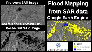
meters depending on the mode it'll provide repeated observations so have a 12-day exact repeat and these observations will allow for applications such as ecosystems hazards and disaster monitoring that include ecosystem disturbances ice sheet collapse natural hazards such as earthquakes volcanoes landslides floods etc next i'll show you a demo on flood mapping using google earth engine so what we'll be doing here is using sentinel 1 sar images to map flood extent in an area in the east coast of the united states this area was flooded by a major hurricane called hurricane matthew back in 2016. so

the approach here is to use google earth engine to run a classification a supervised classification and i'll walk you through each of the steps but before that i'll provide some context about the sentinel 1 images google earth engine is a great resource it's a cloud-based geospatial processing platform platform it's available to scientists researchers and developers for analysis of different ecosystems on our planet in order to use it you do need to have an account but it is free to open one up google earth engine contains a catalog of satellite imagery and geospatial data sets including

sentinel one it has the entire sentinel one database so once you have an account open this is what the google earth engine code editor looks like it's based on javascript there are different windows and the actual you've got the actual code editor in the middle and you can save any sort of code that you write you can search for data sets there's a help button there's a task manager and many different options as explained here so it's a matter of exploring there is a steep learning curve but once you are familiar with the code and

all of the different options embedded into google earth engine it's really a wonderful resource and the best way to become familiar with it is just to practice and explore writing your own code the sar database on google earth engine contains uh the sentinel one and it's uh as mentioned um previously it's a sar sensor operating at c band and it's a satellite from the european space agency so they've got sentinel 1a data and sensor 1b data they are exactly the same satellites with the same sensor each satellite has a global coverage of every 12 days

and so between the two of them you get you get global coverage every six days sentinel one has different modes of operation as listed here there's the extra wide swath mode and that's for monitoring oceans and coasts there's a strip mode and that's by special order only and it's intended for special needs like disasters then there's the wave mode which is intended for oceans and finally there's the interferometric white swath mode which makes routine collections over land and this is the one you want to use for flood mapping [Music] so if you go to the

link indicated here you can access a page containing a description of the sentinel one catalog on google earth engine and this page explains the different modes of images housed on google earth engine as described in the previous slide all the images are in grd meaning they are in the ground range projection they are amplitude images there are no phase images on google earth engine just amplitude images now depending on the mode they might come in different polarizations and resolutions the processing applied was done using the sentinel toolbox and they've applied a thermal noise removal radiometric

calibration and terrain correction so these images are all analysis ready images the only thing you will need to do is to apply a speckle filter and i'll show you how to do that as part of this demo our demo will be focused on a case study in south carolina which is a state on the east coast of the united states a hurricane called matthew made landfall in this state in south carolina as a category 1 hurricane late in the morning of october 8 2016. this hurricane was the most powerful storm of the 2016 atlantic hurricane

season and it cost millions of dollars worth of damage all right so now let's start with the demo let's go through the sequence of steps that need to be applied to the image in order to generate a land cover classification on flooding so this powerpoint slide describes the sequence of steps first you load the images or images to be classified so we'll be filtering through the sentinel one database and identifying the images over our area of interest before the events and after the event then we need to gather the training data so what we'll be

applying here is a supervised classification approach and when you're doing a supervised classification you need to train your classifier so we'll be collecting training data to teach the classifier what are the statistics for each class that we identify and we'll be collecting representative samples of backscatter for each land cover of interest then we'll create the training data set that means we'll overlay the training areas over the images of interest and we'll extract the backscatter for those areas we'll train the classifier and we'll run the classification so in this case we'll run a cart classification and

then finally we'll validate the results and in addition to this we will also overlay population density data and we'll overlay roads data and that's for you to know how to do this and be able to merge different data layers so that then you can really identify areas at risk or whatever your specific application might be if you want to identify perhaps roads that might be inundated or in areas that might be the most suitable roads that might be the most suitable to exit the area that's the way to do it to overlay these different layers

and then i'll finish off showing you how to export the data sets created onto your drive you can follow along with the demo for this part as well as the other two parts tomorrow and thursday by using the software that's indicated on the training web page so this includes the sentinel toolbox and creating an account with google earth engine instructions are included there and the recordings of each part will be made available on youtube within 24 hours after each demo for you to go through at your own pace all right so let's start by identifying

the area of interest and we'll go to your google earth code editor so first of all we'll identify our area of interest by we'll select here the draw a line icon okay and we'll just draw a line more or less over our area of interest so that includes the city of charleston and south carolina here's the city of charleston and let's just do something along these lines here okay and then you go up here this is the polygon that we just identified click on it click on the wheel and change the name from geometry to

roi so that is now officially our region of interest that's where we want to focus okay so next we load the images or images to be classified so let's copy this code and we paste it on our code editor okay so what this is saying is we are searching the database for sentinel one images sorry images so remember this is a c-band sensor and all of the images have been processed as discussed previously and they are in log scale so they are in db these images and so we're going through the collection the copernicus sentiment

one image collection these are grd they're in ground range and we'll filter according to the instrument mode we talked about the interferometric wide swath mode that's the one we're interested in and we'll do an orbital properties pass so we'll we'll look at ascending images the resolution is 10 meters we want to do the search within our area of interest that we define as roi and we want vv and vh images all right so then we filter by date and we display the images on a map so let's just copy this and go back to our

code editor and just copy and paste so we're filtering this sentinel one collection even further we're filtering it to a time frame before the event so we're saying all right before the event was what are the images between october 4th and october 5th 2016 and the actual event what are the images between october 16th and october 17th 2016. okay and then we display these on the map so let's just run this and if you go to layers on the on on the right on the top right here on the map you've got your two mosaics

right so there are two mosaics created before the events and after the event so let's click on before the flood and that's a strange looking image so let's just go in click on the cog there and the reason it looks colored is because there are three images here it's it's it's doing an rgb we have two polarizations vv and vh so it's doing an rgb of vv vh vh so let's just visualize this image just one so let's just visualize the vv and we'll select one band image and you can select either vv or vh

let's just start with the vb we'll do apply all right so that's how our vv image looks like before the event all right so now if you remember the theory that we've covered you can just visually interpret this and identify areas that are urban so you know that urban areas are dominated by double bounds so all of these really really bright white areas those are urban areas that's the city of charleston here and you know that the really dark areas that's open water so you've got inland water here and then you've got the ocean water

and there is some level of roughness obviously that's caused by the wind and that might cause some confusion in the classification this is vv with vh that water is probably going to look really really dark and then we'll we see a lot of features here in the image you see the these areas these are brighter those look like the flood channels and then you've got these darker areas and then here along the coast looks like there's some mangroves here along the coast all right so let's for kicks let's visualize the vh before the event and

here we're stretching the image according to the the range and this stretch is is adequate for vv but not for vh so let's just stretch this a little differently remember uh vh the values tend to be lower so let's just stretch it from minus 25 to five minus five there we go uh we can see you can see that the open water is consistently dark so that's that's where vhs can really make a difference in separating open water from everything else if that's what you're interested in all right so now let's close this and let's

unclick this and visualize after the flood again we go through the same process one band bv let's take a look okay wow you can visually already see some differences here and let's take a look at the vh you can see there's quite a bit of flooding these bright areas remember that's double bound so that's flooded vegetation so this is coastal vegetation that's flooded after the event let's apply the same stretch here for vh minus 25 to -5 and see how that looks so the vh is not picking up that flooded vegetation as well let's try

minus three all right so now let's go back to the vv reset the range here let's go minus 15 and zero okay and what you can do is you can overlay these so let's uh let's do this before the flood let's look at vv and let's do -15 and 0 apply close so if you select both of them you can kind of overlay them and you can control that how you overlay it with this little option up here next to the name of the image so that's before and that's after and that gives you a

sense a clear sense of the differences between those two events those two images but really what's really popping out are those coastal areas how inundated those are all right so let's do this again so you see these these coastal areas and even these these channels you can see that they're brighter after the event than before the event everything in general is probably brighter there's greater reflectivity because things are wetter in general so even though things are might not be inundated in some places it's just generally wetter so it's always good to go through these exercises

just to get a sense of how the images looks like and the differences between the images all right so now let's go on to the next step okay so the next step here is applying a speckle filter and then displaying the filtered image so let's just copy this code and paste it on our here we go all right so what we're doing here is we're applying a speckle filter as you know one of the issues with radar images is that you've got the speckle effect which is this graininess effect and that's inherent of radar images

so in order to reduce that speckle you need to apply a filter if you don't apply a filter your classification will probably look a little grainy okay and there are different size filters obviously the larger the the window that you define the more averaging you do this the smoother things become but you also are losing information you're losing spatial resolution the bigger that window is here we're applying just a simple um just a simple averaging filter smoothing filter and we're displaying the filtered images so that's just zooming in you can see the the speckle clearly

here in the this image now let's apply the filter so you can get a sense on how that image is going to look so let's just run all right so here we have now we have four images before the flood after the flood now before the flood filtered and after the flood filter so let's just take a look at look for comparison after the flood let's go back uv apply and close that so this is the non-specific speckle filtered image and then now let's take a look at after the flood again we go vv apply

close so here you can overlay the original image the non-filtered image that's what it looks like and the filtered image so there is a difference right it is much smoother the filtered image much less grainier okay so now let's move on to the next step which consists of selecting the training data okay so we need to train the classifier and that involves collecting representative samples of backscatter for each land cover class of interest so let's go display the vv image the after vba image filter one and start identifying our our classes so let's do this

and let's do this so you go to geometry imports and you select new layer and a new layer will pop up and we will draw a polygon to identify our new class and let's just call this class permanent water so here here's what we do this is our first class we'll call it open water permanent and then let's represent this class with a blue color just to make things intuitive and where it says geometry import system select feature collection and under properties click on add properties just call it land cover and this class will have

a value of one okay so you'll do the same thing for each class that you define you'll call it uh you you'll define it as a feature collection you'll call it land cover and then the number of the class will will be the the next one so the next class will be class number two etc so let's just do this okay and then select water bodies that or water areas that are permanent water bodies right so the ocean that's permanent that hasn't changed let's go and here where this is an example we're doing this visually

but if you have any sort of training data or data that's been validated that you know for sure those are the conditions on the ground obviously that's always much better i mean how well you train your classifier is really going to make the difference in your results so yeah there's the old saying garbage in garbage out all right so let's just train here that's open water it's always good to pan around the image and try to select different areas are open water just to make sure you have a representative sample of open water so we

know these main river channels those are permanent those are the those were there before and after the event and okay so then we'll define a new class and how do we know those are permanent okay well you you take a look at the before and after and so you overlay them there you go and let's just pan around and take a look at the image all right there you go there so you can clearly see which are the water bodies that are new that weren't there before the event and are now there after the event

so what we'll do is we'll train will actually identify a class as new open water okay so let's just you can zoom in here and sometimes it takes a little while for the images to load as you're zooming in so you have to be patient and that's exactly what's happening here right now so let's just let it load usually there's a bar up here that tells you whether the image is loading or not okay so there and so all of this area is now flooded after the event so let's just go in our new class

let's call it open water flooding okay again geometry feature collection land cover and this is our second class and okay so let's just identify it's one so every time you move around and you want to select a new polygon you have to go in here and and click on it so this is a new body of water okay so so now let's keep defining our classes and the next class to define is flooded vegetation so let's go here and add new layer so we will call the next class quadratic vegetation and make this bright pink

feature collection again land cover and this is going to be our third class so let's pan around here and i identify those areas that were flooded all of these this all of this flooded vegetation here these mangrove areas so let's go in select flooded vegetation and draw a couple of polygons around here okay so let's move on to our next class we'll call that urban so let's make urban nice yellow color and land cover and this will be our fourth class all right so let's identify now the urban areas and here we'll really have to

zoom in so this is an urban area if you're unsure you can again go back to the before the flood and you'll see that the urban areas are continued to be very bright so you might notice that there's a really bright spot here in the middle of the river it's probably a ship okay so let's identify a couple of these all right and one more all right so we've identified these classes and for in the interest of time i've identified two other classes the flood channel and low vegetation so i've done this already let me

just zoom in so you can have a sense of what i've identified i've cut i've created a class called flood channels and those are the brighter areas so those are if you look across the image you have these what i'm um these brighter areas i'm calling those the flood channels so these are the light greens and then i have another class a sixth class called low vegetation and those are the dark green areas so those are the darker the lower back scatter areas they might not necessarily be low vegetation they have just low back scattered

they're probably drier areas so so you define all of your classes you go through the singing process for all of them here you you just add a new layer you make sure you identify it as a feature collection called land cover and then identify the class number so let's go back to our powerpoint and once you've done that then what you need to do is you need to merge the collections into a single collection and and that's called a feature collection so what we need to do is we need to run this piece of code

just copy this and bring it to your code editor and paste it i've got it in here already so i'm not going to paste it i'm just going to uncomment it all right so we've got the code here and what that does is we're calling we're calling new fc that has all of our classes so you need to identify all of the classes that you train for and you need to make sure that you like you give it the same name that you trained for okay if there's the name is off if you've got an

extra letter it's gonna cause an error when you run the classification so we have six classes here are six classes open water permanence open water flooded flooded vegetation urban flood channel and low vegetation and so you've got all of those six classes named here all right so the next thing to do is let's go back here to our powerpoint so now we'll use this feature collection to extract the backscatter values for each line cover class identified in the images that will be used in the classification so what we need to do is we need to

overlay the training data on our image and extract those statistics and so to do that then we take this code and paste it on our text editor so we define the bands to be used to train our data so let's just i've got it here already let's just uncomment okay so what we're saying is make sure that you we're telling the algorithm to extract the backscatter statistics for each land cover class for these two bands vv and vh for our before filtered image or mosaic and after filtered mosaic okay so here we're telling it use

both of these mosaics and vv and vh so remember in in total we have four bads we have two polarizations for each mosaic and we're using all of those to extract the training statistics and to run the classification on all right so the next step is to train the classifier and there are different classifiers that we can use in this case we're using carts which is classification and regression trees so copy this and take it to your editor and what this is doing is we're telling it to use cart to train the classifier okay so

we've got the the training data use the training data land cover so all of our classes that it's a feature collection called land cover and use all of the bands that we identified so we identified vv and bh right so make sure you you save and you can run nothing's going to happen yet so the next step is to run the classification so in the powerpoint i've got a it's just a simple one-liner that runs the classification so we've trained the classifier now we run that on all of the pixels of the images that are

being input into the classifier okay and that would be copy this and also copy this code here so this displays the classification so let's go back and let's just unselect this okay okay so what we're doing now is we're telling a branded classification with all bands and generate a a classification it's called classified not very original name you can name it whatever you want and then display the results display the classification and what this is doing is we're setting the palettes the colors for the different classes that we identified and there are some weird uh

codes here that is coming directly from the colors that we assigned so each color has a color code that's associated with it that's the color code so what i did was i copied that code for each class and i pasted it here so there are one two three four five six different color codes that we're identifying here so let's just start let's save this and let's run okay so that is our classification we've got now five bands here to display we're displaying classification it's not perfect as i said i mean you you really do need

to meticulously define your training areas to get a nice classification but we're picking up the what i call the flood channels we're picking up the flooded areas here in along the coast there's some noise here between what we defined or what i defined as open water and flooded open water and we're picking up the urban areas those are the yellow areas here so this can certainly be refined you can play around whether you want to use just one band up here bb or or vh or if you want to use two bands again you can

play around with the classifier if you want to use a different classifier uh there are lots of options but this just kind of walks you through the steps so so you know what the the process is okay so now the next thing we want to do is we want to create a confusion matrix so we want to really assess the accuracy of our results and what we'll be doing here in this example is we're assessing the accuracy of the training data to determine how well the the the the results how good the results are yeah

how well the classifier performed so what this is doing is it's taking up part of the training data and it's using those to to validate to create this this confusion matrix so for a true validation accuracy you actually want to select two different um samples okay so you've got your training samples and you've got your test samples that's really what you want to do so you copy this code create a confusion matrix and let's go back i've got it here deselect and let's run it and see the results so it's telling us that the classification

accuracy is 87 0.87 and then it's giving us here the confusion matrix so the way to read this is so it's got seven you've got seven values here starting from zero all right so basically it's telling us here that all of the pixels that were identified as permanent open water were classified as permanent open water for this validation the ones that were identified as open water flooded so that would be this class here that would be the second the second class it's telling us that these number of pixels were classified as flooded vegetation urban into

these other classes right so the third class that we identified which was flooded vegetation so most of the pixels were classified as flooded vegetation but there were misclassifications as flood channels or what was called low vegetation okay and so on so what we identified as urban this is indicating that everything that was identified as urban was actually classified as urban in the validation again for a true assessment of your classification accuracy you do have to select independent test data all right so but that gives you a general an assessment of how well your a quantitative

assessment of how well your classifier performed so now in addition to this you can also do other things since google earth engine has several different databases you can overlay different types of data sets on your final product and so what i've done here is i've pulled in a population data so maybe if you're looking at areas if this is a disaster and you want to take a look at populated areas that were flooded or population density you can overlay this layer and to do that you copy this code let's just let's save this and run

it and so what we're doing now is we can overlay population density information so this is a population density layer and so within your area of interest you know as a a disaster manager for example you know then which areas you want to really focus on and another interesting data set that i thought would be very useful especially for disaster related applications is to add a road layer and there is such a database at least for the united states on roads and that's called a tiger dataset so we save this and we run it and

this might be might take a little while because it is it is a very large data set but while that is running let me just show you the different data sets that you can pull if you scroll down here under scripts you've got a list of all of the different data sets that you can pull in so here we have the population density population count you've got the satellite data sets you've got environmental data sets uh you've got topography lithology landforms so there's a lot that you can explore in terms of overlaying your data sets

and the one that contains the roads is the tiger data set so here we have this this is the one that we use tigers 2016 roads you can also overlay like county boundaries state boundaries etc so this roads data set is a big a bit of a large data set and every time you zoom in it just takes a little while to to load up so that gives you a sense then of just the type of things that you can overlay depending on on your interest so so these are all the roads uh really a

lot of detail all right so let's go back now the final step is saving the image so how do you export your results right so copy this there are different ways to export you can use in this example we're exporting to our google drive or to your google drive individual google drive and so let's just copy this and go back here we're exporting as a geotiff and let's just save and then run and what you do is so here's the image we're calling it flooding and that's going to go on your google drive and you

run and a window pops up so this is the name of the image if you want to create a specific folder to put it in oh sorry this is the task name this is the file name we're calling it flooding which is called vlogging hurricane matthew and you run it and it will then save this on your drive so you go into your drive and it should be there as a geotip okay so hopefully this uh has just given you an overview and idea of the steps that you need to go through in order to

generate a classification in this case a classification of flooding flooding extent and this is all a matter of practicing you can play around with things different options just to see what gives you the best results the nice thing is things run relatively quickly and all of the data sets are there already on google earth engine so you can overlay a lot of different data sets on your final product for ancillary information okay so with that i conclude this this first part of this webinar series don't forget that we have two other parts to this tomorrow

december 4th we'll have our second webinar and that will be taught by dr eric fielding from jpl and that one will be about landslide observations using using interferometrics are on what on thursday december 5th we'll have the third part of this webinar series focused on how to generate a digital elevation model and that one will be taught by nikolas gruenfeld from the konai which is the argentinian space agency so we're very excited about having these two guest speakers and about the topics they'll be covering for any contacts questions you can send me an email or

anyone else on this list don't forget that the material is going to be available online the recordings and the presentations will be online for you to be able to go through these there'll be one homework associated with this webinar series and we will assign that homework on the last day and now we'll open up our question and answer session so please type your questions into the box and we'll get to them one by one thank you very much okay so let's start with the questions we've written down your questions on the doc that you see

on the screen all right so question number one which method of water body extraction approach pixel-based object-based or water index gives one the best results in case of using sar hmm i haven't conf can compare different methods and i think this would depend on the size of your water bodies so for example maybe if you have a small river that kind of appears and disappears you might want to do some sort of object-based approach so i think it's something that you'll have to explore to see which yields the best results question two is there a

standardized correction for the effect of incidence angle variation is it applied to google earth's sentinel image library so there are many different ways of doing incidence angle correction with mixed results and the the google earth engine does not apply in incidence angle correction this is not something you need to do in order to um to do analysis with the images necessarily you might have to cut the edges so if the incidence angle variation is too obvious and you can see it visually you can see it or you can look at the pixel values on the

edges of the image then just just cut off the edges and focus on the the middle part of the image so the interferometric white swath mode images their incidence angle varies from about 29 degrees to around 46 degrees all right question number three what are the possible reasons for not forming a perfect interferogram in a low vegetation high perpendicular baseline and good temporal resolution terrain that's a great question and the next two webinars are going to be focused on insar and they will cover this this issue that you just asked and we'll have two experts

on insar tomorrow we'll have dr eric fielding talking about landslides and on thursday we'll have nikolas grunfeld on how to generate a digital elevation model question number four by texture do you mean something like glcm heralic measures yes absolutely that's what i mean and the snap software has texture measurements or texture options that you can generate for your image so i suggest you play around with those and see how well you can how or how much better you can separate some classes that might have confusion uh if for those of you using mv there are

also texture measures in envy and there are probably other texture measures that you can apply using open source softwares like r or grass or geodes or yeah or grass sorry okay the next question how does one detect vegetation inundation in densely populated urban areas in this tutorial the brightness value for urban and vegetation inundation is the same that's right so it's it's difficult and that's why in this theory part i included a short discussion on sources of confusion in when detecting inundated vegetation and that's urban because it's the same backscatter mechanism you've got that double

bounce mechanism and so you have double bounds in areas where there's inundated vegetation and you've got double bonds in areas where there is in urban areas right so you can detect inundation in urban areas and areas where say there are no tall buildings for example so you urban areas you've got a lot of green areas you've got parks and golf courses and and um and fields and so in those areas you can detect um inundation either as open water or inundated vegetation it's just a matter of of knowing where those areas are so you can

properly classify or train your classifier so that's one of the reasons that radar is really not that totally effective in looking at inundation in urban areas just because you already have double bounce as as a dominant backscatter mechanism in in urban areas okay question number six how long does it take to get a google earth agent account accepted have been waiting since the last webinar in early september and still they have not approved my account so it should not take that long in fact it should be a 24-hour thing so if you've been waiting since

september then there's certainly an issue maybe the the email the confirmation email went to your spam or folder so you might want to try again or check your spam folder question number seven can you explain about green space analysis hmm i don't think i understand what is meant here by screen space analysis so you'll have to maybe write out what you mean by green space analysis if if you mean areas where there's vegetation and what sort of analysis are you referring to if you're talking about greenness then radar is not sensitive to the chemical properties

of the vegetation for that you would use something like ndbi or some other measure of greenness question number eight is it possible to overlay roads and other infrastructure data with your flood extent layer outside of the us and google earth engine for example using open street map data i i believe so yes so as you saw there is a database of what is currently sitting in google earth engine but you can also overlay your own vector files or you can export the product that was generated and imported into your own software like qgis and then

overlay whatever data layer you have question number nine is it recommended to apply a speckle filter when a small area is assessed i think that i think the resultant segmentation would miss data okay so uh you should apply a speckle filter even even if it's a small area what you'll want to do is perhaps play around with the size of the filter and it's always going to be a trade-off here anytime you apply a speckle filter you will lose some resolution right obviously the bigger that filter the more resolution you'll lose however you'll have a

cleaner image and you'll have less of less speckle which doesn't means for a cleaner classification question number 10 is there a possibility to integrate sar data with other freely available data for example landsat 8 and other institute data for better visualization yes yeah absolutely and so in google earth engine for example you do have the landsat 8 database and you can integrate those data sets in fact you can use many different layers and run your classification with different layers you can have optical images and radar images and see how well you can your classification results

are and you can also add in-situ data okay question number 11 what to do if roi is not defined in this scope i'm not sure what that means if if the region of interest is not defined in this scope so basically you're defining the region of interest right so at the beginning we drew a box around our area of interest and that was the ri so i'm not sure what this is referring to maybe you can clarify all right question number 12 with editing the dates can we use this code code script for another area

yes absolutely and the whole idea here is this is just an example of uh what you can do for a given area but you can totally take this script and that's the whole idea take the script and modify it and you can define a different roi your region of interest you can define in the search parameters you can define different before and after dates so uh yes that's the that's that's what we want you to do is to use this code script for other areas and you'll have to play around with it a little bit

to see to make sure that there are images available for the dates that you're defining why are urban areas represented by a white color in google earth engine question number 13. so the reason for this is because urban areas are dominated by double bounce and so there's a really very high return in these areas question number 14 can i add a new layer in order to overlay with my results if yes how uh yes absolutely and we showed this i think someone got very excited about uh what could potentially be done and and that's what

we got to at the end so you can overlay many different layers on your on your generated product question number 15 is sar imagery as shown in this webinar useful to detect and quantify urban flooding to or just flooded vegetation areas um i it's more effective much more effective and in vegetated areas to a certain extent you can look at urban flooding as mentioned it's not so much in the areas where it's densely urban where you have a lot of buildings and roads because those areas are going to be dominated already by double bounce okay

and and you can look at this look at the before and after and you'll see that those very bright areas in the before image are as bright and the extent is about the same in the after image so those areas are sorry is not very effective in densely urban areas but urban areas do have parks and open areas and you can detect whether those areas are inundated whether there's open water so you can look at the before and after and see if there's open water if there's specular scattering say in areas where there's a park

or open areas okay great question question number 16 for one class how many samples should one use that's a great question i mean one of the things that you really need to keep in mind is you need to have a good statistical sampling of each class so if you have five pixels defining your one class that's not a large enough statistical sample so you do you want to select at least on the order of 500 to 1000 pixels and so just select try to select your areas as as pure as possible and try to select

your classes across the image so to make sure that you're characterizing each class throughout its the variability in each class all right question 17 do you need global sar data or more local data okay it totally depends on your your needs right so if you're developing some sort of uh global or regional product you can use data that covers a water wider region if if you need local data you can also just pull data over your localized region so it totally depends the nice thing about google earth engine is that all the data is there

and you can easily do like those global analysis um easily okay so it might take a little while it does run in the cloud but it's much more efficient than doing it on your computer okay question 18 during the merge of two or more images i get some unexpected strips how can i remove those small strips actually there is a code that can remove those strips and i'm happy to pass that to you if you send me an email i'll send you the code question number 19 could you please let us know if the training

sample size would affect the result if so how many training samples are ideal for selection so we touched on this you need a representative sample size so you can statistically describe each class but if yes if you have a training sample size that is too small you they'll definitely affect the results i mean remember your classification is going to be as good as your training data so you might have good representative samples of each class but if your classes are are not very if your your training is not very good if the quality of your

training is not very good your classification is not going to be very good so it's very important to have um institute or some sort of validation data where you know that the training that you're selecting for each class that the pixels the training pixels for each class are representative of your class okay great question how will the classifier 20 question number 20 how will the classifier algorithm differentiate between open water flooded and open water permanent they have the same values they all appear dark that's that's true they all appear dark they have the same values

that's very true except you're using two images here remember you're using the before and you're using the after and you have open water flooded what what i'm calling flooded in the after image not but not in the before image okay so question 21. okay so to close up on question 20 so so the the you you train it you train the classifier uh with these classes with these training classes open water permanent open water flooded that one is in one image and it's not in the other image and so the final result will characterize that

open water flooded question 21 how do you define urban areas hard surface and paved areas so the way i define urban areas are just a very bright backscatter areas that i know are in an urban environment okay and if you have doubts of whether that area of really high bright backscatter is actually urban you can go to google earth engine and see what's there sorry google earth and and look at the the images and see what's there or just look at the before and after and if it's really bright and it's not changing then that

that is an urban area if it's really bright in the areas that you know are urban and it's not changing that that is just a very dense urban area where you have streets and you have buildings that are causing that high back scatter return so question number 22 can we download these data using google earth engine uh yes then that was the last step that i showed you how to download the data how to save and and and then you go to the your google drive and you download the data set from there question 23

can we use this data for our phd research publications i don't see why not you'd have to i suggest you discuss this with your advisor and just make sure that proper credit is given to uh to esa for use of their images as well as google earth engine for providing the platform what is the role question 24 what is the role of sar in river modeling studies i'm not sure this is kind of a broad question but i can tell you that one thing that you can do with sar with radar images is generate a

digital elevation model which shows you um how through changes in elevation uh areas where the likelihood of where water should be routed question 25. oh yeah sorry going back to question 23. in in using this data for phd i mentioned giving credit to esa google earth engine and also copernicus okay question 25 does sentinel also provide dm if yes what is the resolution okay so the sentinel one data that's on google earth engine is analysis ready the only thing you need to do is apply a speckle filter so this data has been radiometrically corrected and

and terrain correct it and to do that terrain correction uh it uses a dm a digital elevation model and it uses uh the srtm i believe it uses the srtm 90 meter dm where available and outside of areas where srtm is not available uses aster so in google earth engine you can download dm it's part of the google earth engine database in fact i believe there are several dm's available on google earth engine and you can use a dm for example as a layer into your classification question 26 is sentinel data available frequently in the

indian region i did that depends on what you mean by frequently so the each sentinel one satellite so there's sentinel one a and b has a 12-day temporal repeat and between the two of them it's about six days and in some regions the coverage is denser than in other regions but i think it it's a matter of doing a just a search through the google earth engine database to see what sort of coverage you have in the indian region question 27 is it possible to have free local sar data for a specific place for example

here in madagascar yeah absolutely so this this data data set this data base is global okay there is sentinel one data over india there is sentinel one data over madagascar i i suggest you go and you query the the database to see what sort of coverage you have in madagascar and it's it's all free all of this data is free so you can access it through google earth engine and work on the cloud or you can you can download individual images and work with them on your computer using the sentinel toolbox okay question 28 what

are the different classifiers and which one performs the best i know we're using cart here uh there are you'll have to go and take a look there's supervised classifications there's unsupervised classifications i suggest uh going with a supervised classification so you those usually give you better results uh random forest tends to perform really well carton and especially random forest question 28 the classification by sar images can be improved using classification by optical images i'm possibly it could possibly be improved i'm not sure i would suggest first playing around with the radar images and maybe generating

some textures perhaps pulling in a digital elevation model and then seeing what sort of results you get and you can also test by bringing in optical data optical will really help in areas where there's confusion with some of the classes that you're defining with the radar data so for example one of the things i talked about in the theory part was that you might have some confusion in areas where there's open water and areas where there's low vegetation or there's like bare soil these areas are dominated by either specular scattering or or just very low

back scatter and so there might be some confusion and optical images might be able to help separate those areas and help clear up that sort of confusion so how many classes would be enough for training in order to get the best results so we've touched on this but now in terms of classes itself it's a matter of it's not really how many classes it you can you can train for many different classes and so even within one class if you see a certain variability within one class you might want to divide it into two you

might want to say well this is bare soil and this is an area with very low vegetation they'll look very similar but they're slightly different and then you can always merge the classes in your final classification if the results are not good yeah and one way to see how well your classes separate or how distinctive they are is to just look at the histogram of your classes look at the the histogram of all your classes and see what sort of overlap they have all right so the next question how does one export the imagery to

using another image processing software okay so at the end i showed you how to save it as a geotiff this then goes into your google drive and you just export that and you can open it in qgis question 32 how to decide on the number of classifications for the study area on the number of classifications i'm not sure i understand this question maybe on the number of classes if so if it is the number of classes it just depends on what you want to classify right now you do want to kind of cover the broad

range of variability in the image so even though you might just be interested say in open water you can't just classify for open water you you want to classify for well all right let's classify for open water and everything else land all right question number 33 i am not clear on what data were used for accuracy assessment usually would use an independent data set how would you input independent data yes so i did this is a very good point and i did mention touch on this briefly but i'm glad you brought it up because you

want to do your accuracy assessment on areas that are independent from your training areas right so if you do your accuracy assessment using the same pixels that you use to train your classifier you're not really getting a true accuracy assessment it's biased right so ideally you want like a a second set of defined classes that you can then use to validate your results and in order to do that it's the same way the same way we created this feature collection and we called it uh land cover uh you again you create one just like that

just call it something else and then when you run the uh the validation you call that validation data set okay question 34 for classification is it mandatory to use polygons or can you actually use point data for instance if you use the point data from a survey like lucas for land cover yeah absolutely you can use point data except the thing the problem about point data it's it's just a point and this goes back to what is an adequate number of samples so you wanna characterize each class in a statistically representative way and if you

have unless you have a lot of lot a lot of point data then that's fine but if you just have a couple of points then that you might not get as very good results okay question 35 are the tiger road maps and the population density only for the us so the population density i believe that is global the tiger roads map i believe that is just for the u.s question 36 will it be correct if i use a mosaic average values of all the s1 images in a month to estimate flooding in that month so

you don't want to use mosaic average values for a whole month just because especially looking at flooding because flooding it can be dynamic and things can change in a relatively short period of time so really doing an average over a month might not give you a representative result of flooding extent question 37 could you send us the polygon so we have the same data set especially for the land cover uh yeah absolutely just send me an email and i'd be happy to send you the polygons so question 38 did you use training samples for validation

how you use validation samples in this case so i think that was answered in the previous question question 39. question 39 all right is it recommended to apply a speckle filter when a small area 14 hectares is assessed i think that the resultant segmentation would miss data the thing about a speckle filter even if it's a small area you still have the effect of speckle will translate into your final classification product so you do want to apply some sort of filter and my best advice is just run it both ways it's very quick especially if

you're working in a relatively small area and and compare the results question number 40 we took to analyze with images with resolution 10 by 10 meter but exports to google drive result image with resolution of 100 by 100 meters why is this uh it might be the way that the export was defined and even though the original image is 10 by 10 meters that the actual resolution is going to be reduced what after you apply the filter question 41 what about doing the same for drought uh yeah that's a a great point actually arsed has

had some webinar series looking at drought and for that you bring in other data sets like soil moisture to look at the extent of of drought and how that's changing with time question 42 how do you remove the wave wind effect on the large open water that's a that's a great question what you do is ideally you want to use the a hv okay because hv is less sensitive to the effects of wind on on water and that confusion then of open water as as land as kind of a bare surface land are the data

sets used in this demonstration global almost all the data sets are global actually so we talked about this the sentinel one is is global the population data is global the tiger data is just for the u.s actually i'm sorry so that the tiger data is a population data set okay sorry i i clarify myself the population data set is global that's not the tiger and then the tiger data set which has the roads that is just for the u.s okay the next question is there any possibility to import external shape files for training yes i

google earth engine has an option to import your own files do i need to learn coding to use this data or are or there are already pre-coded things i can just follow you can you use this code and just modify the code to your area of interest question 46 how can i difference between urban areas and flooded vegetation both are represented by white color so we've addressed this already in previous questions how successful have attempts been to automate these disaster mapping analysis processes question 47 as opposed to case by k spaces is each situation far

too variable to allow automation uh this is a really good question i'm not sure i can fully answer this because i haven't attempted to automate it but i believe there are efforts or out there to to automate the use of star data for disaster mapping and actually a great example of that is the aria project that's a jpl led effort that provides information on on flooding for example and it has done some automation it's still being improved however okay and i think so that's it in terms of oh okay let's let's uh a couple more

questions if included vh in my band selection it fails let me see oh okay so we have a couple more all right if if i include the h in my band selection it fails i'm assuming that polarization isn't available that is correct so it's hv with sentinel 1 it's hv it's uh uh hold on sorry with a sentinel one i apologize iw interferometric white swath is vh and v vv so it should not fail uh i would suggest going back and revisiting your code sometimes they're little things that if you don't have quotes correctly it

will give you an error so make sure your code is correct question 49 how to separate out smooth land areas high specular reflectance from those of surface matter in google earth engine i i'm not sure what is meant here by surface matter question 50 is there any method offered by the google earth engine for mapping flood based on an automatic comparison between the before and after images yeah that's a good question there might be i i i'm not familiar with any but there might be is sar imagery better for agricultural crop classification which band is

good for this purpose that's question 51 that's a great question and yes you can use our imagery to distinguish different types of crops we had a whole session on that the on the last advanced webinar series i suggest you revisit that question 52 is the overlapping of the inundation output from supervised classification with the impossible in google earth engine to get the depth of inundation in flooded areas if so how you can definitely overlap a dm to your inundation classification but in this case you cannot get depth of inundation in flooded areas okay i'll do

two more questions i've seen most of the demonstration lectures in flat areas how do we remove the shadow effect when dealing with flooding classification in the mountainous areas that's a great question and the best way to deal with shadow is just to create a mask and treat it as areas where there's no data question 54 what would be an acceptable sar data latency for real-time disasters that totally depends on the disaster obviously the quicker you have the data the better it is and i'll answer also i i read some comments about why i was using

ascending images the reason i was using ascending is because there was better coverage over this area with ascending images actually there were no images for the time frame that i defined in the for descending passes that's why i use just ascending okay so uh we're a little bit past our our our two hour session i want to thank all of you we'll put the questions online and we'll ask actually finish answering these questions in the document so you can revisit these if we didn't get to your question uh keep tuned because we have two more

uh webinars a great one tomorrow on landslide observations by dr eric fielding and then the one on thursday by nicolas gruenfeld on generating a digital elevation model thank you very much for tuning in for all your questions and we'll be in touch again tomorrow stay tuned you