Lec 4, Central Tendency and Dispersion - I

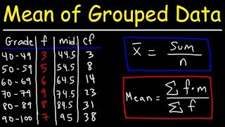
[Music] [Music] [Applause] [Music] [Applause] [Music] good morning students today's we are going to the lecture for in this lecture we are going to talk about central tendency and how to measure the dispersions the lecture objectives we talk about different types of central tendency then different types of dispersions what is measure of central tendency measure of central tendency yield information about particular places or locations in a group of numbers suppose there are a group of number is there that number group of numbers has to be replaced by a single number that single number we can call it as central tendency that is a single number to describe the characteristics of a set of data some of the central tendency which we are going to see in this lecture is arithmetic mean weighted mean median percentile in the dispersions we are going to talk about skewness kurtosis range interquartile range variance standard score and coefficient of variation first we will see the first central tendency arithmetic mean commonly it is called as the mean it is the average of a group of numbers it is applicable for interval and ratio data this point is very important it is not applicable for nominal and ordinal data it is affected by each value in the data set including extreme values one of the problem of the with the mean is that it is affected by the extreme values computed by summing all values in the data set and dividing the sum by the number of values in the data set see here I have used a notation mu mu means capital letters mu represents mean for the population the formula is Sigma X by n that is X 1 plus X 2 plus X 3 and so on plus xn greater by n here n is the number of elements for example the values are 24 13 1926 11 add these numbers and divided by five because there are five elements so $93 by five eighteen point six is the mean of the these five numbers so now the 18. 6 can be replaced by this set five numbers okay suppose in your class if you see the average mark is 60 so the whole marks of the all the students can be represented to be a single number that is 60 60 will give an idea about the performance of the whole class next what is the sample mean make sure that the difference here the x-bar previously for the population mean we have used mu for the sample mean we are using X bar X bar is Sigma X by n X 1 plus X 2 plus external by n for example 6 element is there 50 786 42-38 1966 so divided by 6 the mean is 63 point one six seven now how to find out the mean of a grouped data the mean of your group data is nothing but weighted average of class midpoints class frequencies are the weight for the formula is mu is Sigma F indium graded by Sigma of F here F represents the frequency M represents the midpoint so Sigma F M is nothing but F or M 1 plus F 2 M 2 plus F 3 M 3 and so on plus fi mi da da by sum of all F that is nothing but you are yen we will see you an example see this is the group data what is given class interval is given frequency is given class midpoint is given and multiplied value of frequency and midpoint also we can find out for example C here 20 to 30 there are six number is their frequency 6 suppose if you say the marks of here if you say this this is an example of here marks obtained by near class so between 20 and 30 there are 6 200 there between 30 under 40 there are 18 shoulders there suppose for this if the data is in this format that is in Group D format how to find out the mean okay first what do you want to do rule first you have to find out the class midpoint see 20 to 30 that is a class interval the midpoint is twenty-five for thirty and forty the class midpoint is the middle value 35 like this 45 55 65 75 next one you have two multiplied by frequency and class midpoint so 6 into 25 150 18 into 35 6 30 11 and 45 for 95 and so on what the formula says it is a sigma of FM to draw my sigma f last column the sum value is two one five zero two thousand hundred and fifty divided by fifty Sigma F is some of the frequency so for this kind of grouped data the mean is four to three now we'll go to the next central tendency that is the weighted average some time if you look at the previous values the each values is given equal weight days suppose it is not always the case there may be some marks there some values where there may be higher weight age so for that case we have to go for weighted average some time you see this we will list two average numbers but we want to assign more importance or weight to some of the numbers the average you need is the weighted average so the weighted average is sum of the product of weights and that value greater by sum of values where X is the data value and W is the weight assigned to that data value the sum is taken over all data values we will see one application of this weighted average suppose your midterm test score is 83 and your final exam is score is 95 using weights of 40% is for the midterm and 60% is for the final exam compute the weighted average of your scores if the minimum average for an A grade is 90 will you earn an A grade so first we find out the weighted average so the mark is 83 weight age is 40% age for midterm for interim your mark is 95 wait age is 60 percentage so multiply that then get away some of the weight that is 0. 4 plus point 6 is one so 90.

2 so if you are above 90 you will get a because you are crossing 19 obviously you will get the a greater now we will go to the next central tendency median the middle value in ordered array of number is called median it is applicable for ordinal interval and ratio data you see previously the mean is applicable only for interval and ratio data but the median is applicable for ordinal data there is a point has to be remembered and it is not applicable for nominal data and one advantage of median is it is unaffected by extremely large and extremely small values next we will see how to compute median there are two procedure first two processes arrange the observations in an ordered array if there is an odd number of item the median is the middle term of the ordered array if there is the even number of terms the median is the average of middle two terms another procedure is the medians position of an ordered array is given by n plus 1 divided by 2 n is the number of data set we will see this example I have taken some exam some numbers that is arranged in your order that is an ascending order 3 4 5 7 up to 22 there are 17 terms in the ordered array the position of the median is with respect to previous let n plus 1 by 2 so n plus 1 by 2 17 plus 1 18 der by two 9 so the median is the ninth the term ninth the term here is 15 if see the 22 which is the highest number is replaced by 100 still the median is 15 see if the 3 is replaced by minus hundred and three still the median is 15 so there's the advantage of this median over mean is median is not disturbed by extreme values previously the number of items are R now let us see the another situation there are 16 terms in the ordered array there is an even number the position of the median is n plus 1 by 2 that is 16 plus 1 by 2 is 8 point 5 so we ought to look at the term where it is the the push of 8. 5 that is the median is between eighth and the ninth term here the eighth the term is fourteen nine therm is 15 so average of that one is 14. 5 again if the 21 is replaced by 100 the median is same 14.

5 if the 3 is replaced by minus 88 still the median is 14. 5 now let us see how to find out the median of your group data but it will be group data here if the data is given in the form of a frequency table this case the formula to find out the median of a group data is median equal to L plus n by 2 minus CF Peter by F median material by W where L is the lower limit of the median class before using this formula from the given table you were to find out what is the median class then cfp cumulative frequency of the class preceding the median class F median the frequency of the median class W is the width of the median class n is the total number of frequencies see this is an example as I told you before using this formula first order to find out the median class what is the median classes when you add the frequency it is a 50 c6 plus 18 plus 11 plus 11 plus 3 plus 150 so divide this 50 by 2 it is a 25 in the community frequency column in the last column look at where that 25 is lying it is not between 30 and 40 it is going to lie on between 40 and 50 because 20 for the next term is 35 so the median class for this given group data is 40 and 50 so as usual yell is the lower limit of the median class that is a 40 plus n is 50 50 by 2 - you see the cumulative frequency of the preceding interval is 24 so 50 divided by 2 minus 24 didn't why the frequency of the median class is 1111 W is 10 because the width interval is 10 when you simplify you would get 40 point nine zero nine so this is the way to find out the median of your group the data now mode the most frequently occurring value in your data set is more applicable to all level of data measurement nominal ordinal interval and ratio sometimes there is a possibility the data set may be bimodal bimodal means data sets that have two modes that means two numbers are repeated same number of time multimodal data sets that contain more than two mode see this one sample data as it is given for this data set the mode is 44 because the 44 is appearing more number of time how many number of time 1 2 3 4 5 ok so the mode is 44 that is there are more 40 force than any other values that is the formula for finding mode of your group 2 data here first we have to find out the mode class for that look at the frequency column there 18 is the highest frequency so corresponding the in class interval is called mode interval okay the mode interval LMO is the lower limit of that mode interval is 30 plus the d1 is difference between 18 and 6 and d2 is difference between 18 and 11 see 30 plus say D 1 is nothing but 18 is the mode interval and then the previous frequency is 6 so 18 minus 6 is 12 duder by d1 is 12 plus d2 is the difference between your 18 and 11 that is 7 so 12 plus 7 x width is 10 so 36. 3 1 is the mode of your group data yes we have studied mean median mode for group data and ungroup the data now the question is when to use me when to use median when to use mode okay many time even though we study mean median for we are not exactly told how to use or when to use me or when to use median or when to use mode for example look at this data set this is left skewed data this is left skewed data because the tail is on the left hand side the example for this is suppose say the exam is very easy question paper any x axis is the march in y axis is frequency so there are more number of students who got higher marks where the question paper is easy situation this is an example of left skewed data so what will happen here the here here will be mean here will be median this will be more you see another example where the question paper is very tough so this is called right skewed data you know here what is happening how we are saying that since the question paper is very tough there are more number of students who got the lesser marks that is why the skewness on this side so here there will be mean here will be median this will be more okay there will be another situation it is symmetric it is a bell looking at bill shaped curve in this situation now after looking at this hypothetical problem now the question arises when to use mean when to use median mode look at the location of the median the median is always in the middle whether the data is left skewed or right skewed the median is always the middle so whenever the data is skewed you should go for median as here central tendency if your data is following a bell-shaped curve then you can use mean median mode there is no problem at all the clue for that choosing the correct central is first you have to plot that curve go to plot the data outer plotting the data you have to get an idea of the skewness of the data set how it is distributed whether it is right skewed or left skewed or it is bell shaped curve if it is skewed data you go for median as the center tendency if it is following a bell-shaped curve you go for mean or median or mode as a central tendency now you go to next one is a percentile mainly this you might have seen some of the cat examination scores over gate examination scores their performance is expressed in terms of percentile not the percentage because percentile is having some advantage over percentage because percentage is absolute term but the percentile is the relative term the measure of central tendency that divide a group of data into hundred parts it's called percentile for example somebody say 90th percentile my score is 98 99 90th percentile indicates that at most 90 percent of the data lie below it and at least 10 percentage the data lie above it okay the median and the 50th percentile have the same value it is applicable for ordinal interval and ratio data it is not applicable for nominal data okay we'll see an example how to compute a percentile the first step is organize the data into an ascending ordered array calculate the peak percentage location suppose if I want to know xxx the percent a location for that you have to find out the value I is nothing but P divided by 800 multiplied by n n is the number of data set the I is nothing but the percentiles location we got to find out the I value if I is a whole number the percentage is the average of the values at the I and I plus 1 positions if I is not a whole number the percentile is the I plus 1 position inya ordered array look at this example the raw data is even 14 12 19 up to 17 I have arranged in the ascending order the lowest values file the highest value is 28 suppose I want to know xxx the percentile for knowing the 30th percentile first I have to find out I that is a $32 by 100 meter by 8 so 2.

4 the I is nothing but location index as I explained the previous slide I is not the whole number so you have to add I plus 1 so 2 point 4 plus 1 is 3 point 4 in the 3 point 4 the whole number portion is 3 right so the 30th percentile is at the third location of an array when you look at the third location is 13 that means a person who scored 13 marks his corresponding percentile is 30 so far we talked about these different central tendency will go for differing now we are going for measuring dispersion measures of variability describes the spread or the dispersion of the set of the data the reliability of measure of central tendency is the dispersion because many time the central tendency will mislead the people so the reliability of that central tendency is calculated by are identified by its corresponding dispersion it is used to compare dispersion of various samples that is why whenever you plot the data you not only show the me no to show the central tendency also because the reliability of mean is explained by dispersion you look at this data when you see the first two rows is no variability in cash flow mean is same the second one says variability in cash flow see there is a lot of variability in the second one but the mean is same if you look at only the mean it look like same when you look at only the mean the mean value same but when you look at see the left hand side the second dataset is having more variability the quality of the mean is explained by its variability there is nothing dispersion there are different measures to measure the variability one is the range interquartile range mean absolute deviation variance standard deviation their scores on coefficient of variations we will see one by one suppose there is an group of data is there see this one you have to find out the range the range is nothing but the difference between the largest and the smallest value in a set of data it is very simple to compute the problem here is it ignores all data points except the two extremes so the range is the largest value is 48 in this data set the smallest value is 35 it is only 13 you see that only the two values are taken care in between the values is not taken into consideration for finding the range it is a quick estimate to measure the dispersion of a set of data I will go for your quartile quartile measures the central tendency that divided group of data into four subgroups we say Q 1 Q 2 Q 3 Q 1 is nothing but 25 percentage of the data set is below the first quartile Q 2 50 percentage of the data set is below the second quartile q3 75 percentage the data set is below the third quartile so we can say Q 1 is the 25th percentile Q 2 is the 50th the percentile nothing but the median this is a very important point Q 2 is nothing but the median q3 is the 75th percentile and another point is the quartile value ZAR not necessarily members of the data set you see this let's say say q1 q2 q3 so q1 see first 25 percentage the data set q2 first 50 percent of the data set q3 75 percent of the data set okay it is nothing but the quartile is used to divide the whole data set into four groups first 25 second 25 third 25 and last 25 suppose an example for finding the quartile suppose the data is given 1 0 6 1 0 and so on okay we have arranged it in the ascending order first we got to find out the Q 1 Q 1 as I told you to the about 25th percentile so the location of the 25th percentile first you have to find out the location index I for the 2588 it is a 2 since the 2 is the even number as I explained previously if it is the location takes it - you have to find out that position plus the next position and it's average so in the second positions data set is 1 1 0 9 the next one is 1 1 4 divided by 2 so one hundred eleven point five so the q 1 is nothing but here one hundred and eleven point five Q two 50th percentile 50 divided by 100 multiplied by 8 it is a four again the 4 is the even number so the fourth location is one two three fourth locations 116 and flip the location is 120 one rotor by to 118 point five so the Q to our median is 118 point five then Q 375 divided by hundred melted by eight again six six is the even number the average of sixth and seventh values are 122 + 125 hundred by two so the value is 120 3. 5 this is the way to calculate Q 1 Q 2 Q 3 now the next term is interquartile range so the dispersions in the data set is measured with help of interquartile range by using this formula q3 - q1 as we know Q 3 is 75th percentile q1 is the 25th percentile so range of values between the first and third quartile is called interquartile range it is a range of middle of why we are using quartile range because it is the less influenced by extreme values because when we collect the data set we are not going to consider at very low values at the same time very high values so the middle values which is not affected by extremes that is taken for further calculation for that purpose we are using interquartile range there is a q3 now he'll go for deviation from the mean so dataset is the given 5 9 16 17 18 to find the deviation from the mean first to find the mean mean is 13 suppose there is a graph is there so this is the 13 okay see the first value 5 the difference is 5 minus 13 that's a minus 8 so this distance is your first deviation the second data is 9 so 9 minus 13 is minus 4 this is minus 4 so this deviation is expressed by this lines look at that there is a negative deviation there is a positive deviation suppose if we want to add the deviation general it will become 0 that's why we should go for mean absolute deviation you see this it is given here there are two values are negative deviation there are three values are positive deviation when you add this it is becoming 0 so it seems we are getting 0 we cannot measure the dispersion one way is we have to remove this negatives you take only positive value when you take positive values 24 so 24 data by 5 there are 5 data set so 4. 8 is called mean absolute deviation it is the average of absolute deviations from the mean there was a problem in the mean absolute deviation I will tell you what is the problem there see the next we will see a population variance it is not the average of the squared deviation from the arithmetic mean okay so the X is their mean is there so when you add the absolute even hundred in 0 one way the previously the mean absolute deviation you take an only positive value now we are going to square it the squaring of the deviation having some advantage one advantage is we can remove the negative sign second one is but the deviation is less when you square it for example minus 4 square is 16 C minus 8 squared is 64 so what is happening more the deviation more this squared value okay so here the Sigma square is Sigma of X minus mu greater by X minus mu whole square by n so 130 dotted by five here we are squaring the purpose why we are squaring for there are two reason one is to remove the negative sign the second reason is given for higher penalty for higher deviation values the next one is the population standard deviation because underneath there is a variance but variance is acquired a number that we cannot compare suppose the two numbers are given say 12 and 13 that is easy intuitively we can say which is higher which is smaller suppose 124 169 is given notice quite a number we cannot compare intuitively and not only that it is in the square root of square term we want to have it in the actual term so for comparison purpose for that purpose we are taking square root of that so 5.