Lec 14: Confidence interval estimation: Single population - I
34.58k views3489 WordsCopy TextShare

IIT Roorkee July 2018
Confidence Interval Estimation, Point estimate, t distribution, Z distribution, Single population pr...
Video Transcript:
Welcome students to the next lecture. Today lecture is we are going to talk about the confidence interval estimation for the single population. In the previous lecture, we have seen the sampling distribution.
Sampling distribution we have seen three results, out of the sampling distribution lecture. One is sampling distribution for mean, sampling distribution for proportion and sampling distribution for variance. By using that result we are going to estimate some population parameters.
What we are going to estimate? We may estimate the mean of the population or the proportion of the population or the variance of the population. That we will see in this lecture.
The objective of this course is to distinguish between a point estimate and a confidence interval estimate and construct and interpret a confidence interval estimate for a single population mean using both Z and t distributions. Today also in this lecture I am going to introduce Z and t distribution then, form and interpret, a Confidence Interval estimate for a single population proportion, create confidence interval estimate for the variance of the normal population. In the confidence interval, what we are going to see today confidence intervals for the population mean there are two possibilities: When the population variance Sigma square is known, other case is when population variance Sigma square is unknown.
Then, confidence interval for the population proportion is P hat, using large samples. Then, confidence interval estimate for the variance of your normal distribution. Before getting into the content, we will see what is the estimator and estimate.
An estimate of your population parameter is a random variable that depends on sample information. An estimator whose value provides an approximation to the unknown parameter for example, a specific value of the random variable is called estimate. For example X bar is estimator for population mean.
Similarly S square, sample variance an estimator for population variance P hat, population proportion is estimated for P hat normal proportion is estimated for population proportion. So, this X bar s square P hat these are called estimator. A specific value of x bar, s square, P hat is nothing but estimate.
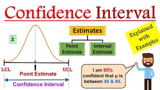
In estimate, there are two things we can say, one is a point estimate is a single number other one is a confidence interval provides additional information about the variability. We can say it is a point estimate and interval estimate because in point estimate is only single number. It is not very much reliable but the confidence interval is giving you additional information about the variability of that point estimate.
For example when you look at this picture, we say what is a point estimate and interval estimate. A point estimate is a single number and interval estimate provides additional information about the variability of the point estimate. For example, you see that if I, if I say tomorrow what is going to be temperature if I say is exactly 35 degree Celsius, this is a point estimate.
If I give some lower limit and upper limit for this for example, this may be say 30 to 40 that is the confidence interval. And I say 35 it is a single number but when I say 30 to 40 that is in confidence interval. So, the 30 can be called as a lower confidence limit the right side can be called as upper control limit 40.
So this is width of confidence interval the point estimate is just one number, single number. Yes, so, point estimate we can estimate population parameter mean mu with the help of sample mean that is x-bar. We can estimate population proportion P with help of sample proportion small p.
Then, another important property of this estimator is it should be Unbiasedness. A point estimator theta hat is said to be an unbiased estimator of the parameter theta if the expected value or mean of the sampling distribution theta hat is theta. So, then we can say it is unbiased estimator if the expected value of theta hat equal to theta, then, we can say it is the unbiased estimate.
For example if I say X bar then when I can say X bar is an estimator of population proportion. If I say, if the expected value of X bar is equal to mean then we can say X bar is an unbiased estimator, the sample mean X bar is an unbiased estimator for mu the sample variance small s square is an unbiased estimator for Sigma square, the sample proportion small p is an unbiased estimator for population proportion P. Look at the, another property of unbiasedness.
Suppose, if you look at this picture, there are two pictures there. One is for theta one another one is theta two. So, theta one the mean of theta one cap is nothing but your theta.
So, the theta one cap is an unbiased estimator. But theta two cap is not unbiased estimator because the mean will be somewhere here, because it is not the population mean, let us see the unbiasedness of an estimator. There is a two figure is there.
One is theta 1 hat another one is theta 2 hat. If you look at the theta 1 cap the mean of theta 1 cap is the theta that is the population mean. But the mean of theta 2 cap is away from the population mean.
So, we can say theta 1 cap is an unbiased estimator of the population. We can measure the biasness. Let theta hat be an estimator of theta the bias in theta hat is defined as the difference between the mean and theta.
So, the biasness of theta cap is nothing but the expected value of theta hat - theta. The bias of an unbiased estimator is 0 if it is 0 we can say there is no biasness. How can we see the most efficient estimator?
Suppose there are several unbiased estimator of theta, we have seen sample mean is the one of the estimator of the mean. The most efficient estimator or the minimum variance unbiased estimator of theta is the unbiased estimator with the smallest variance. So, even though there are different estimators to predict the population parameter, we have to see a estimator which is having the smallest variance is the efficient estimator.
Let theta 1 hat and theta 2 hat be the two unbiased estimator of theta. Based on the same number of sample observation then theta 1 hat is said to be more efficient then theta 2 hat, variance of theta 1 hat is less than the variance of theta 2 hat. So what is the point here is there may be different estimator for the population parameter if we want to say which is more efficient we have to see the variance of the estimator.
If the variance of the estimator is lesser then that estimator is the most efficient estimator. The relative efficiency of theta 1 hat with respect to theta 2 is the ratio of their variance. So, relative efficiency is variance of theta 2 hat divided by variance of theta 1 hat.
Then, Confidence Interval. How much uncertainty is associated with the point estimate of the population parameter because when I say, the previous example the temperature is 35 degree how much uncertainty is associated with that point estimate. That uncertainty is expressed with the help of confidence interval.
An estimate provides more information about the population characteristics than does a point estimate. So, when compared to point estimate, interval estimate is giving more information about the population. Such interval estimates are called confidence intervals.
So, for example, if we say this is the population I am taking different sample say, the population mean may be say 40. I have taken various sample with help of sample mean, I can predict what will be the lower limit and upper limit of this population mean. For example, if I say, 35 to 45 this interval is nothing but confidence interval.
I can go for an exactly endpoint estimate for example if I exactly I can say, point estimate is I can say, exactly say, 40. But the 40 is not much reliable. Confidence interval estimate: An interval give, gives you a range of values.
And confidence interval takes into consideration, variation in sample statistics from sample to sample, because what will happen, if there is a big population, we may take different samples but different sample may have different variance, we are constructing the confidence interval with the help of that variance. So the consideration for the sample to sample is taken with help of, taken into account with help of confidence interval. We can construct the confidence interval based on observation from one sample for example, if we say X bar with the help of one sample, I can predict what is the upper limit and lower limit of your mu.
It gives information about closeness to unknown population parameters. Stated in terms of level of confidence, can never be 100Percentage confident. We cannot be always 100 Percentage confidence.
Let us see what is the confidence interval and confidence level? So, confidence interval is lower limit and upper limit, the confidence level is nothing but the probability. If P (a less than THETA less than b) = 1 - Alpha then the interval from a to b is called 100 into 1 – alpha, confidence interval.
So, this interval a to b is taken as the confidence interval. The quantity 1 - alpha is called a confidence level. So, confidence level is a probability confidence interval is the lower limit upper limit of population proportion.
So the confidence level alpha is between 0 and 1. In any repeated samples of population the true value of the parameter theta would be contained in 100 (1 – alpha)Percentage of intervals calculated this way. The confidence interval calculated in this manner is written as a less than THETA less than b with 100 ( 1 – alpha)Percentage confidence level.
Next we will see what is the estimation process? Look at this the left-hand side this is the whole population mean mu is unknown. We want to predict what is the value of the mean.
So, you take the sample the green one say the sample mean is 50, with the help of the sample mean you can say what is the lower limit and upper limit of this population parameter mu, with a certain level of confidence. Say I am saying I am 95Percentage is confident that the Mu is between 40 and 60. Then we go to what is a confidence level suppose confidence level is 95 also written as 1 - alpha.
We will see in detail what is alpha. Alpha is called a type 1 error. So, 1 - alpha is 0.
95, a relative frequency interpretation from a repeated samples 95Percentage of all the confidence intervals that can be constructed will contain the unknown true parameter. So, what is the meaning of this 95Percentage is, even though we will see in the coming slides. Suppose if you construct an interval with some range say 40 to 50.
So what is the meaning of this 95Percentage so, this interval when you repeat this experiment 100 times, there is a 95Percentage of time you can capture the true mean within this interval. Only 5Percentage of the time this true mean may be outside the interval okay. A specific interval either will contain or will not contain the true parameter.
For example, this interval sometime may contain true parameter otherwise may not contain the true parameter. But when is a 95 Percentage 95 Percentage of the time this interval can't the true parameter there is only five Percentage turns this interval will not capture the true parameter. The general formula for confidence interval is point estimate is, general formula for point estimate is nothing but your x-bar + or - this reliability factor we will see later, Z.
This is standard error. If you use a standard error, Sigma/Square root n, so x-bar + or - Z (Sigma/Square root n) is nothing but the formula for confidence interval. So, when you say + it is upper limit if it is - it is lower limit.
The value of the reliability factor depends upon the desired level of confidence. The value of Z is depending upon how much confidence level you need to have that we will see. So, the confidence intervals we will see the classification.
We can find the confidence interval for the population mean, we can find confidence interval for the population proportion, we can find the confidence interval for the population variance. In this population mean, there are two category one is Sigma square that is the population variance is known, Sigma square is unknown, the population variance is unknown, whenever the Sigma square, whenever there is a capital letter that represents about the population; whenever there is a small letter that represents about the sample. We will see first one confidence interval for Mu.
That means we are going to find the confidence interval of population mean. First case is the Sigma square is known. Sigma square is population standard deviation is known.
What assumptions? Population variance Sigma square is known. Population is normally distributed.
If the population is not normal, we have to go for large sample size use a large sample. So, the confidence interval estimate is X bar - Z alpha by 2 Sigma by root n less than mu less than X bar + Z alpha by 2 root of Sigma divided by root n, where Sigma Alpha by 2 is the normal distribution value. So, this is nothing but it will be like this, right.
So, this one has come from this formula X bar - Mu Sigma/ root n. When you when you re-adjust this equation you can find the MU upper limit. This is upper limit, lower limit okay.
When you re-adjust this, Z alpha by 2 is nothing but because we are finding both the sides, so this value is alpha by 2. This value is alpha by 2. So, the remaining places that is 1 - alpha.
So, this 1 - alpha is called Confidence interval. We will say one more term called margin of error. The Confidence interval X bar - Z alpha by 2 Sigma by root n less than Mu less than X bar + Z alpha by 2 Sigma by root n can be written as X bar + or - ME.
This ME is nothing but margin of error. So, this term, so this term we can call it as margin of error. You should be very careful when we say, error; generally, another name for standard deviation is the error.
Therefore if we write Sigma by root n that is standard error if we say Z alpha by 2 Sigma by root n that is a margin of error. All our error, error is nothing but the variation. So, this is error this is we can say this is error.
This is standard error, this is margin of error okay. The standard error whenever you go for sampling that Sigma has to be divided by root of n. This is the result of central limit theorem okay.
Generally, we have to look for reducing the margin of error. The margin of error can be reduced by looking at this Sigma, n and Z. If the population standard deviation can be reduced when you reduce Sigma, obviously, margin of error will reduce.
When you increase the sample size we can predict more accurately the error can be minimized. So, the margin of error will be minimized okay. What is the meaning of this one is, suppose this is one confidence level, this is another confidence level.
For this margin of error for this one, margin of error is more this one, margin of error is more for this one, the margin of error is more. What do I mean whenever the confidence level is small, the margin of error also reduced. Then, we look at how to find out the reliability factor that is Z alpha by 2.
For example, if I suppose, if you want to know something at 95Percentage confidence level, so this is 95Percentage confidence level so the remaining is 5Percentage, when you divide this 5Percentage by 2 see the right hand side you will get is 0. 025. The left hand she will get 0.
025. When you look at the Z table, when the right hand side is 0. 025, the corresponding Z value is 1.
96 on right hand side. The left side it is - 1. 96.
This z 1. 96 is called upper confidence limit. The left hand side it is called lower confidence limit.
The value of Z has to be captured by looking at what is the alpha value. So, when you look at the table the Z value, for 0. 025 is + or - 1.
96 is from the standard normal table. This we can find out. Look at this, suppose, if the confidence level is 80Percentage.
This is nothing but 1 - alpha. When you look at the table it is 1. 28.
But it is at 90Percentage, 0. 90 when you look at the table it is 1. 645.
Generally we will go for 90, 95, 99. So, this value can be remembered. Most of the time, we will go for 95, if it is 95, the Z value is 1.
96. Z alpha by 2 not exactly Z, it is Z alpha by 2 when it is 99 then the confidence coefficient - alpha is 0. 99 then Z alpha by 2 value is 2.
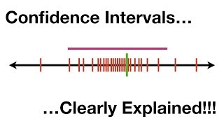
58. Next we will see intervals and level of confidence. As I told you, you see that so I have captured 7 intervals.
Out of 7, one interval is not lying you are not able to capture the blue one. We are not able to capture the true population parameter okay. So, this is nothing but confidence interval.
So, this portion is nothing but your confidence level. So, 100 (1 – alpha) Percentage of intervals constructed contain mu, that is 100 alpha do not. Interval extended from lower control limit is X bar - Z Sigma by root n upper control limit is X bar + Z Sigma by root n.
This we can say this is nothing but your X bar + Z Sigma by root n. This left hand side is X bar - Z Sigma by root n. If I say 95Percentage level of confidence what is the meaning is, if I constructed it 100 times, out of a 100 times, 95 time my interval which I have constructed will capture the true population mean.
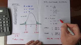
Only 5Percentage of time it may not capture the true population parameter. Example a sample of 11 circuits from your large normal population has a mean resistance of 2. 20 ohms.
Here the sample value is given. This is your sample mean is given. We know from the past testing that the population standard deviation is 0.
35 ohms. Determine 95Percentage confidence interval for the true mean resistance of the population. So, what is a given is this is n, this is your 2.
20 the sample mean. So, x-bar is given 2. 20, + Z because the Z value which we got from the table because it is a 95Percentage is confidence level.
But it is a 95 Percentage confidence level then, the Z value is 1. 96 Sigma value is 0. 35 is given.
There are 11 samples root of n. so, when I say this one the lower limit is 1. 9932, the upper limit value is 2.
4068. So, how we are to interpret this is, we are 95Percentage confident that the true mean resistance is between 1. 9932 and 2.
4068 ohms. Although the true mean may or may not mean in this interval. 95 Percentage of intervals formed in this manner will contain true mean.
Only 5Percentage of time this may not have the true mean. That is called your significance level. Another name is called type 1 error.
Another name is called producers risk. This will see in detail in coming lectures ok. We will go to the next category.
We will predict the confidence interval or the mean when Sigma square that is the population variance is not given. Dear students I will summarize what we have done so far. We have seen what is the point estimate; we have seen what is the interval estimate we have seen advantage of interval estimate then, we have seen what is the meaning of confidence level.
Then confidence interval after that we have seen how to predict the confidence interval of a population mean when Sigma square is known. In the next lecture will go for predicting the population mean when Sigma square is unknown, thank you.
Related Videos
![Confidence Interval [Simply explained]](https://img.youtube.com/vi/ENnlSlvQHO0/mqdefault.jpg)
5:34
Confidence Interval [Simply explained]
DATAtab
530,931 views

1:08:17
Hypothesis testing (ALL YOU NEED TO KNOW!)
zedstatistics
284,523 views

2:24:10
Statistics Lecture 7.2: Finding Confidence...
Professor Leonard
317,429 views

28:19
Lec 6, Introduction to Probability-I
IIT Roorkee July 2018
98,838 views

26:35
Lec 14: Employee Recognition - II
IIT Roorkee July 2018
698 views

7:40
Confidence Interval for a population mean ...
Joshua Emmanuel
87,772 views

1:18:03
1. Introduction to Statistics
MIT OpenCourseWare
2,029,420 views
8:24
Confidence Interval in Statistics | Confid...
Digital E-Learning
248,826 views

29:02
Concept of Confidence Interval and Examples
Dr. Harish Garg
43,651 views

42:09
Teach me STATISTICS in half an hour! Serio...
zedstatistics
2,751,282 views
14:47
Confidence Intervals In Statistics- Part 1
Krish Naik
142,374 views
3:20
How to Calculate Confidence Interval in Ex...
Maven Analytics
15,511 views

20:08
Why the p-Value fell from Grace: A Deep Di...
DATAtab
108,060 views
6:44
Confidence Interval for a population propo...
Joshua Emmanuel
70,411 views
44:47
Theory of Estimator| Point and Interval Es...
Dr. Harish Garg
121,031 views
6:59
How To...Calculate the Confidence Interval...
Eugene O'Loughlin
565,920 views
6:42
Confidence Intervals, Clearly Explained!!!
StatQuest with Josh Starmer
338,814 views

2:26:50
Statistics Lecture 8.2: An Introduction to...
Professor Leonard
565,087 views

30:04
ANOVA (Analysis of Variance) Analysis – FU...
Green Belt Academy
90,599 views