Do stock returns follow random walks? Markov chains and trading strategies (Excel)

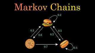
hello everyone and welcome again to nettle the best platform around for distance learning in business finance economics and much much more please don't forget to subscribe to our channel and click that bell notification button below so that you never miss fresh videos and tutorials you might be interested in we would also greatly appreciate if you consider supporting us on patreon so please check the link in the description for more details my name is sava and today we're discussing yet another test for market efficiency that can be used to determine if stock prices follow random walks but unlike the previous tests we have discussed in previous videos like runs test or variance ratio test this one is quite a bit more flexible and can be much more easily translated into trading strategies that can be used to exploit the inefficiencies you discover and gain you potentially some abnormal profits this test utilizes the logic of markov chains markov chains are a very useful tool in mathematical statistics and probability theory that is crucial in interpreting and visualizing probability the logic of the test is that you take some daily data or any period data on the returns of your financial instrument of choice and in our case it is as usual the returns of s p 500 index over a five year period from the start of 2015 all the way down to end of 2019 and to apply the markov chains test for market efficiency you have to separate those stock returns into states and calculate the probabilities of transition from one state into the other what exactly are states well it's perhaps the easiest to conceptualize states when considering the simplest case with two states and here markov chains test can remind you of the runs test consider this let's separate our stock returns into stock returns above zero and below zero and name those states one and two respectively then we can calculate the probability of the stock return moving from state one to state one so moving up after moving up in the previous day and the probabilities of transition from states one to two two to one and two to two so respectively what is the probability of the stock price going down after it went up of it going up after it went down or of it continuing going down after it went down in the previous day but you don't need to stop there you can consider more states than two you can separate your stock return data into equal sub samples based on the value of the magnitude of the return and calculate what are the probabilities of the stock return transitioning from one state into the other in the following day so how to apply it mathematically well first of all we have to calculate the empirical distribution of stock returns and it has to deal with ranks of our stock returns in the overall sample so we can first of all just calculate the rank and here it's the best to calculate average ranks however it doesn't really matter you can also opt for equal ranks the results would not differ much and we just need to calculate the rank of a particular observation in the whole array of stock returns and this array has to be locked because we don't want it to change observation to observation and we need to rank our stock returns in the ascending order from lowest the most negative to highest the most positive so we input one over here and then we have to divide it by the total number of observations we're having and you can easily verify it using the count function for example that the total number of stock returns in our five-year trading period is 1258 so this easy procedure will give us the empirical distribution function for the stock returns of s p 500 and now based on these values of the empirical distribution function we can sort our stock returns into states and here i'll consider three examples with two three and four states respectively here we need to apply some neat mathematical tricks using excel formulas but bear with me it would be really intuitive when we get through it to separate our stock returns into two states we need to consider stock returns below and above the median so we can just apply the round down function and apply it to our value of the empirical distribution and we have to lock the column here because we will drag it around for different numbers of states and we don't want it to change in terms of the column and multiply it by the number of states and here we have to lock the row because we want the column to change as we move to an example with a different number of states but we don't want it to change when we move from observation to observation within one example with a particular number of states and we need to round it down to the nearest integer so the number of digits is zero because we're not concerned with the decimal expansion we're concerned just with the integer because we want to separate them into states one and two and the final problem is that we have got an example when our value of the empirical distribution function is equal to 1 which is the highest value of our stock return throughout the period the maximum so we have to subtract 1 if our product of the empirical distribution function and the number of states is wholly divided by one so here if mod which is the remainder of whole division of the same expression mod c3 times g2 which is the empirical distribution function times the number of states divided by one is equal to zero we have to subtract one and leave it as it is if it's not the case and here we will get a value of the function that will give us zero or one if we have two states zero one or two if we have three states and zero one two or three if i have four states and so on and so forth if we were considering examples with even higher number of states and finally we have to add one so that our uh state uh ids are natural numbers so starting with one not starting from zero so that's just the technical uh complication here that is easily accounted for by just adding one to the formula so we can enforce this formula drag it across the total number of states and bottom right click it all the way down for all of our observations and we can see that this neat formula has allowed us to sort our stock returns into two three or four states respectively for example the stock return of 1. 34 that occurred on the 16th of january 2015 is so high that is first of all the 95th percentile of the empirical uh distribution which can be considered quite high historically and we can see that our procedure has sorted it into the second state in the example with two states third and fourth in the examples with three and four states respectively so always it classifies it into the state with the highest return so bear this in mind in our case the higher the number of state the higher is the return that's what we will be interested in when formulating potential market beating trading strategies and for example uh the other way around on the 27th of january 2015 the return was 1. 34 percent which was the approximately the sixth percentile of the empirical distribution function and we can see that regardless of the number of states it always sorts it into the first state so the state that is characterized by the lowest returns the most negative returns that have been observed during this observation period so now we have to actually calculate the transition probabilities or the number of realizations of a particular event of a particular transition so here we have already got some table templates set up so for the case of two states we will just need to calculate the number of occurrences when an observation of state 1 is followed by an observation of state 1 an observation of state 2 is followed by the observation of state 1 and so on and so forth so basically it calculates how likely it is that a particular transition occurs so without further ado we can just apply the count ifs function and count how many times we have got our observation of a particular state and here we have to get all the way down except for one last observation and we need to lock both the column and the row in its array so we need to count how many times our initial observation falls within the first state and here we need to lock the column but not the row how often is it followed by the observation from the first state as well so here we have to select the area starting from the second observation because the first is already been taken and get all the way down to the very end and here we also have to lock it all both columns and rows and refer to the one at the top and here we also need to lock the row but not the column so applying this quite bulky yet quite intuitive function we can count how many times is a one followed by a one and dragging it across and down we can see how frequent are those transitions we can see that it's more likely that a one will be followed by two and it's more likely that the two will be followed by one while other things held equal so we already can notice some inefficiencies some predictability but how significant are these inefficiencies these discrepancies we would expect if the market was perfectly efficient that those two values and those two values would be equal because it wouldn't matter what happened before in terms of what would happen tomorrow so to compare this with some expected scenario that we would have expected if the market was perfectly efficient we can calculate the expected uh occurrences of such transitions and apply the well-known chi-square test to calculate how significant is the deviation from the expected outcome and we have already got a separate video that when we explain the logic and the application of the chi-square test so here we'll cover it just briefly to calculate the expected number of transitions uh in a particular row that basically is a transition following a particular state that has been realized in the past we can just calculate the average over all elements of a particular row and given the fact that we will apply it for multiple examples with two states three states and four states we can just calculate the average of this array with empty elements so that we could copy it across and not bother ourselves with typing the formula over and over again given the fact that excel recognizes empty cells as blanks and doesn't consider them towards the calculation of the average and the only thing we need to do here is to lock the columns but not the rows obviously and apply the formula and drag it across and down so we can see that here we would have expected an observation of state 1 to be followed by 313 observations of both state 1 and 2 and it quite significantly deviated from the reality but to formalize our hypothesis testing we have to calculate the chi squared statistic and we can actually do it in one go here we can just apply the sum function and sum the square deviations of the observed values from the expected values so this array minus that array squared divided by the uh occurrence of the expected values over here and that gives us our chi squared stat and we have to reinforce this formula and shift ctrl enter as this formula deals with subtracting and dividing a bunch of matrices so we can press shift ctrl enter and get our chi-squared stat of 2.

63 approximately how significant is this chi squared stat well to do that we have to apply the chi-squared uh right-tailed distribution input the value of the chi squared statistic as our x and number of the degrees of freedom would be the product of the number of rows minus one and the number of columns minus one here we've got two states two columns minus one times two states two rows minus one so simple as that so it will give us a one degree of freedom in the end so we enforce this formula and we can see that our p-value is 10. 51 percent which is alarmingly low but not low enough to reject the null hypothesis of efficiency to reject the null hypothesis that the market is indeed efficient and that's that and that the transitions from one state into the other are random but what will we see when we increase the number of states we consider well to easily apply it for more and more examples we can copy this formula paste it into that cell drag the respective arrays to the column that corresponds to the number of states equal to three and drag these cells to the ones corresponding to a particular identifiers of a state given this example and we can enforce this formula again drag it across and down and get our observed occurrences of transitions from one state into the other and here given the fact how smartly we applied this average formula we can just copy this formula across without tweaking anything and drag it throughout the whole table and again we can apply the chi-squared stat subtracting the expected occurrences from the observed occurrences square this difference and divided by the matrix of the expected occurrences close the parentheses and enforce this four moves and shift ctrl enter and get a quite higher chi squared stat of 9. 4 but bear in mind that we have also increased the number of our degrees of freedom as we consider three states instead of two states so all other things held equal we would have expected our chi squared stat to be higher even though the deviation might have been perfectly random so now we have to apply the chi-squared right-tilt distribution again input our new chi-squared stat as the x-value and the new number of the degrees of freedom that would be the total number of columns minus one times the total number of rows minus one and we enforce this formula and get five point eighteen percent which is lower than ten percent so we can say that this deviation from market efficiency this deviation from randomness of transition probabilities is significant at ten percent but not significant enough to be significant five percent but it's indeed alarming we can already see that given three transition states we can already pinpoint some notable deviations from perfect randomness but what would happen if our number of transition states would increase further to four well we already know what to do we can copy this formula over here drag the arrays to the new column drag these cells down apply the formula drag it across and drag it down and we see that quite naturally the number of observations in each of these cells decreases further and further as we increase the number of states and that's the ultimate limit of the markov chains test because for the chi-squared test to be powerful enough you need to have at least 30 observations in each of your cells because chi-squared test behaves very badly in small samples so you can increase your number of states quite far down the line but bear in mind that if you start encountering values lower than 30 in your cells your test stops being that reliable but here we can also apply the formula for the averages for the expected occurrences drag them across the table and apply the well-known formula for the chi-squared stat observed minus expected squared divided by expected and enforcing it using shift quarterly answer and we've got a chi squared stat that's uh yet greater still and converting it into a p-value using the appropriate number of degrees of freedom number of columns minus one times the number of rows minus one we get a p value of 5.

5 percent which is again close to what we've obtained in the previous example but a little bit higher so here we can reasonably assume that we would not actually spot anything more significant than five percent if we further increase the number of states and given the fact that our number of observations in each of the cells uh approximately comes uh alarmingly close to 30. we can stop our testing here but if you have larger samples you can proceed with the test in the similar fashion to five six or even more states and that's what's beautiful about it the flexibility and the nature of the test that you can test for a multiple number of ways that the market can be inefficient that is what differs it from runs test or variance ratio test again but now and that's arguably what is the most exciting about markov chains test is that we can look closely at those transitions occurrences and formulate some plausible strategies that could exploit the inefficiencies we have spotted at least at the significance level of 10 first let's consider the example with three transition states for this example we can see that the most striking uh occurrence is that it is much more likely to get a three so very high return after you've got a very low return in the start so actually this uh transition matrix tells us well it's probably good to invest in the market when it just went down by a lot when the past transition state is one it's likely that the next transition state would be three so we'll gain if you invest at that point and let's just test that let's consider that we are a very cautious investor and we only want to invest when we are more likely to gain and let's do just that so here we see that we have to invest or we are better off investing when the past state was equal to one and we are doing it in the example with three states so let's apply this strategy simulation so let's think about what our strategy implies our strategy implies that if the past state is one so if the stock market fell by a lot in the previous day we are likely to get a higher attendant the next day so we would invest so it means that in the next day we would obtain the return of the market if on the other hand we get states of two or three in the past day uh there are no uh notable patterns that are beneficial for us well if the state was two it's quite a bit less likely that you get a high return so it's kind of disadvantages us and if the state number is three we can see that the probabilities are even more even so you are not getting anything in terms of the gain over the market so in that case the investor can just stay in cash and obtain a secure return of zero at that particular day so let's apply this strategy all the way down for all of our trading days and see how well did it perform to do that we can just compare the return of our strategy and the risk of our strategy to that of the market to that of the s p 500 index to calculate the annualized return of the market we can as usual apply the product one plus function um and apply it to the whole area of market returns and given the fact that we've got five years worth of data we have to raise it to the power one-fifth and subtract one to get the return and not the rate of appreciation and enforce this formulation shift control answer we get that the average return of the market annualized during that period was 9. 42 which is pretty typical of um u.

s stock market uh for annualized risk we can apply the sample standard deviation function and apply it again to the whole array and to annualize it we can multiply by the square root of 252 and we can see that the market provides us with an average annualized return of 9. 42 subject to risk of 13. 4 percent but what about our strategy let's apply the same formula product one plus to the area of our strategy returns that will include zeros when we didn't invest because we believed in our markov chain strategy and uh equal to the market return when we believe that investing is beneficial and well likely to obtain a high return so here we just do the same thing and raise it to the power one fifth and subtract one and we see that we have obtained a little bit lower incentive that of the market but bear in mind we have devised the strategy for a cautious investor but maybe there are some gains in terms of the risk we're exposed to let's test that let's calculate the standard deviation of the returns of our strategy and multiply it by the square root of 252 and we can see that indeed we have reduced our risk quite a lot from 13.

4 to 9. 4 percent and we have sacrificed only a little bit of return for obtaining this particular gain in terms of risk so for some risk-averse investor such a strategy could be profitable obviously if you can trade at reasonably low trading costs but we have got another potential candidate for a profitable strategy if we look at the example with four states we can see that here the case that the market is more likely to go up by a lot after it fell by a lot is even more prominent you are much more likely to transition from stage one from state one into state 4 than all other 3 states so we can apply this logic and simulate another strategy by just tweaking it a little bit and referring to a different column if our state number in the previous day was equal to one when we have four states invest and don't invest and stay in cash if your state number is anything but one because we can see here that there are um no potential uh gains that are as high as for the state number of one if we are currently at states two three or four so the logic actually kind of persists from the previous example let's see what this strategy delivers let's enforce this formula and bottom line all the way down and all the formulas would be recalculated automatically and we can see here that this strategy delivers even lower return but it also reduces risk but the reduction of return from seven to five percent is quite material it's comparable to the decrease in return we have um experienced when uh opting for the markov chain strategy with number of states equal to three but the reduction of risk is not that material from 9. 4 to uh 8.